Chapter 15 Bayes factors

This chapter is based on a longer manuscript available on arXiv: Schad, Nicenboim, Bürkner, Betancourt, et al. (2022b); our terminology used here is based on the conventions used in that paper. A published version of the arXiv article appears in Schad, Nicenboim, Bürkner, Betancourt, et al. (2022a).

Bayesian approaches provide tools for different aspects of data analysis. A key contribution of Bayesian data analysis to cognitive science is that it furnishes probabilistic ways to quantify the evidence that data provide in support of one model or another. Models provide ways to implement scientific hypotheses; as a consequence, model comparison and hypothesis testing are closely related. Bayesian hypothesis testing comparing any kind of hypotheses is implemented using Bayes factors (Rouder, Haaf, and Vandekerckhove 2018; Schönbrodt and Wagenmakers 2018; Wagenmakers et al. 2010; Kass and Raftery 1995; Gronau et al. 2017; Jeffreys 1939), which quantify evidence in favor of one statistical (or computational) model over another. This chapter will focus on Bayes factors as the way to compare models and to obtain evidence for (general) hypotheses.

There are subtleties associated with Bayes factors that are not widely appreciated. For example, the results of Bayes factor analyses are highly sensitive to and crucially depend on prior assumptions about model parameters (we will illustrate this below), which can vary between experiments/research problems and even differ subjectively between different researchers. Many authors use or recommend so-called default prior distributions, where the prior parameters are fixed, and are independent of the scientific problem in question (Hammerly, Staub, and Dillon 2019; Navarro 2015). However, default priors can result in an overly simplistic perspective on Bayesian hypothesis testing, and can be misleading. For this reason, even though leading experts in the use of Bayes factor, such as Rouder et al. (2009), often provide default priors for computing Bayes factors, they also make it clear that: “simply put, principled inference is a thoughtful process that cannot be performed by rigid adherence to defaults” (Rouder et al. 2009, 235). However, this observation does not seem to have had much impact on how Bayes factors are used in fields like psychology and psycholinguistics; the use of default priors when computing Bayes factors seems to be widespread.

Given the key influence of priors on Bayes factors, defining priors becomes a central issue when using Bayes factors. The priors determine which models will be compared.

In this chapter, we demonstrate how Bayes factors should be used in practical settings in cognitive science. In doing so, we demonstrate the strength of this approach and some important pitfalls that researchers should be aware of.

15.1 Hypothesis testing using the Bayes factor

15.1.1 Marginal likelihood

Bayes’ rule can be written with reference to a specific statistical model \(\mathcal{M}_1\).

\[\begin{equation} p(\boldsymbol{\Theta} \mid \boldsymbol{y}, \mathcal{M}_1) = \frac{p(\boldsymbol{y} \mid \boldsymbol{\Theta}, \mathcal{M}_1) p(\boldsymbol{\Theta} \mid \mathcal{M}_1)}{p(\boldsymbol{y} \mid \mathcal{M}_1)} \end{equation}\]

Here, \(\boldsymbol{y}\) refers to the data and \(\boldsymbol{\Theta}\) is a vector of parameters; for example, this vector could include the intercept, slope, and variance component in a linear regression model.

The denominator \(p(\boldsymbol{y} \mid \mathcal{M}_1)\) is the marginal likelihood, and is a single number that gives us the likelihood of the observed data \(\boldsymbol{y}\) given the model \(\mathcal{M}_1\) (and only in the discrete case, it gives us the probability of the observed data \(\boldsymbol{y}\) given the model; see section 1.7). Because in general it’s not a probability, it should be interpreted relative to another marginal likelihood (evaluated at the same \(\boldsymbol{y}\)).

In frequentist statistics, it’s also common to quantify evidence for the model by determining the maximum likelihood, that is, the likelihood of the data given the best-fitting model parameter. Thus, the data is used twice: once for fitting the parameter, and then for evaluating the likelihood. Importantly, this inference completely hinges upon this best-fitting parameter to be a meaningful value that represents well what we know about the parameter, and doesn’t take the uncertainty of the estimates into account. Bayesian inference quantifies the uncertainty that is associated with a parameter; that is, one accepts that the knowledge about the parameter value is uncertain. Computing the marginal likelihood entails computing the likelihood given all plausible values for the model parameter.

One difficulty in the above equation showing Bayes’ rule is that the marginal likelihood \(p(\boldsymbol{y} \mid \mathcal{M}_1)\) in the denominator cannot be easily computed in Bayes’ rule:

\[\begin{equation} p(\boldsymbol{\Theta} \mid \boldsymbol{y}, \mathcal{M}_1) = \frac{p(\boldsymbol{y} \mid \boldsymbol{\Theta}, \mathcal{M}_1) p(\boldsymbol{\Theta} \mid \mathcal{M}_1)}{p(\boldsymbol{y} \mid \mathcal{M}_1)} \end{equation}\]

The marginal likelihood does not depend on the model parameters \(\Theta\); the parameters are “marginalized” or integrated out:

\[\begin{equation} p(\boldsymbol{y} \mid \mathcal{M}_1) = \int p(\boldsymbol{y} \mid \boldsymbol{\Theta}, \mathcal{M}_1) p(\boldsymbol{\Theta} \mid \mathcal{M}_1) d \boldsymbol{\Theta} \tag{15.1} \end{equation}\]

The likelihood is evaluated for every possible parameter value, weighted by the prior plausibility of the parameter values. The product \(p(\boldsymbol{y} \mid \boldsymbol{\Theta}, \mathcal{M}_1) p(\boldsymbol{\Theta} \mid \mathcal{M}_1)\) is then summed up (that is what the integral does).

For this reason, the prior is as important as the likelihood. Equation (15.1) also looks almost identical to the prior predictive distribution from section 3.3 (that is, the predictions that the model makes before seeing any data). The prior predictive distribution is repeated below for convenience:

\[\begin{equation} \begin{aligned} p(\boldsymbol{y_{pred}}) &= p(y_{pred_1},\dots,y_{pred_n})\\ &= \int_{\boldsymbol{\Theta}} p(y_{pred_1}|\boldsymbol{\Theta})\cdot p(y_{pred_2}|\boldsymbol{\Theta})\cdots p(y_{pred_N}|\boldsymbol{\Theta}) p(\boldsymbol{\Theta}) \, d\boldsymbol{\Theta} \end{aligned} \end{equation}\]

However, while the prior predictive distribution describes possible observations, the marginal likelihood is evaluated on the actually observed data.

Let’s compute the Bayes factor for a very simple example case. We assume a study where we assess the number of “successes” observed in a fixed number of trials. For example, suppose that we have 80 “successes” out of 100 trials. A simple model of this data can be built by assuming, as we did in section 1.4, that the data are distributed according to a binomial distribution. In a binomial distribution, \(n\) independent experiments are performed, where the result of each experiment is either a “success” or “no success” with probability \(\theta\). The binomial distribution is the probability distribution of the number of successes \(k\) (number of “success” responses) in this situation for a given sample of experiments \(X\).

Suppose now that we have prior information about the probability parameter \(\theta\). As we explained in section 2.2, a typical prior distribution for \(\theta\) is a beta distribution. The beta distribution defines a probability distribution on the interval \([0, 1]\), which is the interval on which the probability \(\theta\) is defined. It has two parameters \(a\) and \(b\), which determine the shape of the distribution. The prior parameters \(a\) and \(b\) can be interpreted as the a priori number of “successes” versus “failures.” These could be based on previous evidence, or on the researcher’s beliefs, drawing on their domain knowledge (O’Hagan et al. 2006).

Here, to illustrate the calculation of the Bayes factor, we assume that the parameters of the beta distribution are \(a=4\) and \(b=2\). As mentioned above, these parameters can be interpreted as representing “success” (\(4\) prior observations representing success), and “no success” (\(2\) prior observations representing “no success”). The resulting prior distribution is visualized in Figure 15.1. A \(\mathit{Beta}(a=4,b=2)\) prior on \(\theta\) amounts to a regularizing prior with some, but no clear prior evidence for more than 50% of success.

FIGURE 15.1: beta distribution with parameters a = 4 and b = 2.

To compute the marginal likelihood, equation (15.1) shows that we need to multiply the likelihood with the prior. The marginal likelihood is then the area under the curve, that is, the likelihood averaged across all possible values for the model parameter (the probability of success).

Based on this data, likelihood, and prior we can calculate the marginal likelihood, that is, this area under the curve, in the following way using R:⁵⁰

# First we multiply the likelihood with the prior
plik1 <- function(theta) {
  dbinom(x = 80, size = 100, prob = theta) *
    dbeta(x = theta, shape1 = 4, shape2 = 2)
}
# Then we integrate (compute the area under the curve):
(MargLik1 <- integrate(f = plik1, lower = 0, upper = 1)$value)

## [1] 0.02

One would prefer a model that gives a higher marginal likelihood, i.e., a higher likelihood of observing the data after integrating out the influence of the model parameter(s) (here: \(\theta\)). A model will yield a high marginal likelihood if it makes a high proportion of good predictions (i.e., model 2 in Figure 15.2; the figure is adapted from Bishop 2006). Model predictions are normalized, that is, the total probability that models assign to different expected data patterns is the same for all models. Models that are too flexible (model 3 in Figure 15.2) will divide their prior predictive probability density across all of their predictions. Such models can predict many different outcomes. Thus, they likely can also predict the actually observed outcome. However, due to the normalization, they cannot predict it with high probability, because they also predict all kinds of other outcomes. This is true for both models with priors that are too wide or for models with too many parameters. Bayesian model comparison automatically penalizes such complex models, which is called the “Occam factor” (MacKay 2003).

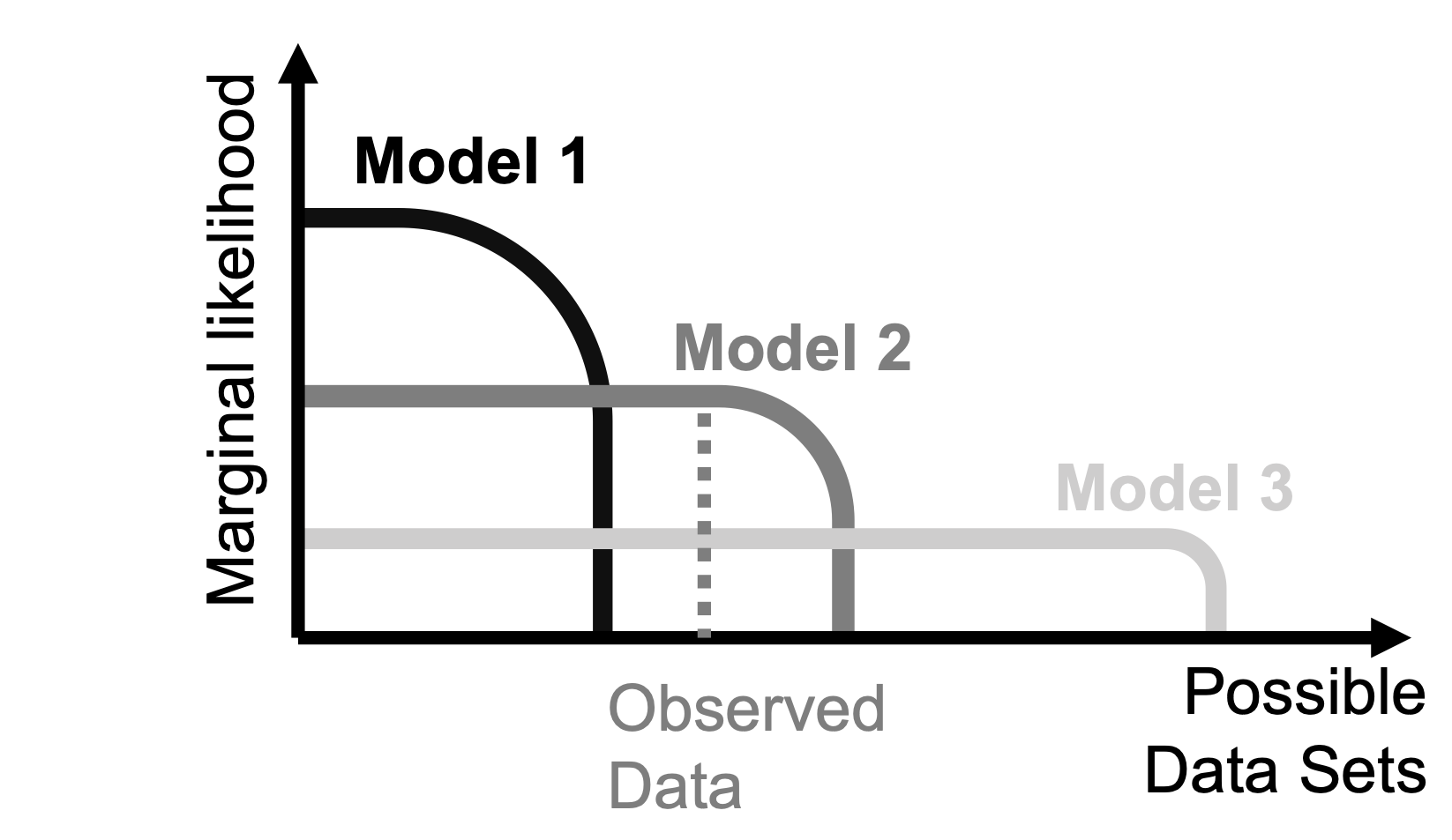
FIGURE 15.2: Shown are the schematic marginal likelihoods that each of three models assigns to different possible data sets. The total probability each model assigns to the data is equal to one, i.e., the areas under the curves of all three models are the same. Model 1 (black), the low complexity model, assigns all the probability to a narrow range of possible data, and can predict these possible data sets with high likelihood. Model 3 (light grey) assigns its probability to a large range of different possible outcomes, but predicts each individual observed data set with low likelihood (high complexity model). Model 2 (dark grey) takes an intermediate position (intermediate complexity). The vertical dashed line (dark grey) illustrates where the actual empirically observed data fall. The data most support model 2, since this model predicts the data with highest likelihood. The figure is closely based on Figure 3.13 in Bishop (2006).

By contrast, good models (Figure 15.2, model 2) will make very specific predictions, where the specific predictions are consistent with the observed data. Here, all the predictive probability density is located at the “location” where the observed data fall, and little probability density is located at other places, providing good support for the model. Of course, specific predictions can also be wrong, when expectations differ from what the observed data actually look like (Figure 15.2, model 1).

Having a natural Occam factor is good for posterior inference, i.e., for assessing how much (continuous) evidence there is for one model or another. However, it doesn’t necessarily imply good decision making or hypothesis testing, i.e., to make discrete decisions about which model explains the data best, or on which model to base further actions.

Here, we provide two examples of more flexible models. First, the following model assumes the same likelihood and the same distribution function for the prior. However, we assume a flat, uninformative prior, with prior parameters \(a = 1\) and \(b = 1\) (i.e., only one prior “success” and one prior “failure”), which provides more prior spread than the first model. Again, we can formulate our model as multiplying the likelihood with the prior, and integrate out the influence of the parameter \(\theta\):

plik2 <- function(theta) {
  dbinom(x = 80, size = 100, prob = theta) *
    dbeta(x = theta, shape1 = 1, shape2 = 1)
}
(MargLik2 <- integrate(f = plik2, lower = 0, upper = 1)$value)

## [1] 0.0099

We can see that this second model is more flexible: due to the more spread-out prior, it is compatible with a larger range of possible observed data patterns. However, when we integrate out the \(\theta\) parameter to obtain the marginal likelihood, we can see that this flexibility also comes with a cost: the model has a smaller marginal likelihood (\(0.0099\)) than the first model (\(0.02\)). Thus, on average (averaged across all possible values of \(\theta\)) the second model performs worse in explaining the specific data that we observed compared to the first model, and has less support from the data.

A model might be more “complex” because it has a more spread-out prior, or alternatively because it has a more complex likelihood function, which uses a larger number of parameters to explain the same data. Here we implement a third model, which assumes a more complex likelihood by using a beta-binomial distribution. The beta-binomial distribution is similar to the binomial distribution, with one important difference: In the binomial distribution the probability of success \(\theta\) is fixed across trials. In the beta-binomial distribution, the probability of success is fixed for each trial, but is drawn from a beta distribution across trials. Thus, \(\theta\) can differ between trials. In the beta-binomial distribution, we thus assume that the likelihood function is a combination of a binomial distribution and a beta distribution of the probability \(\theta\), which yields:

\[\begin{equation} p(X = k \mid a, b) = \frac{B(k+a, n-k+b)}{B(a,b)} \end{equation}\]

What is important here is that this more complex distribution has two parameters (\(a\) and \(b\); rather than one, \(\theta\)) to explain the same data. We assume log-normally distributed priors for the \(a\) and \(b\) parameters, with location zero and scale \(100\). The likelihood of this combined beta-binomial distribution is given by the R-function dbbinom() in the package extraDistr. We can now write down the likelihood times the priors (given as log-normal densities, dlnorm()), and integrate out the influence of the two free model parameters \(a\) and \(b\) using numerical integration (applying integrate twice):

plik3 <- function(a, b) {
  dbbinom(x = 80, size = 100, alpha = a, beta = b) *
    dlnorm(x = a, meanlog = 0, sdlog = 100) *
    dlnorm(x = b, meanlog = 0, sdlog = 100)
}
# Compute marginal likelihood by applying integrate twice
f <- function(b) {
  integrate(function(a) plik3(a, b), lower = 0, upper = Inf)$value
  }
# integrate requires a vectorized function:
(MargLik3 <- integrate(Vectorize(f), lower = 0, upper = Inf)$value)

## [1] 0.00000707

The results show that this third model has an even smaller marginal likelihood compared to the first two (\(0.00000707\)). With its two parameters \(a\) and \(b\), this third model has a lot of flexibility to explain a lot of different patterns of observed empirical results. However, again, this increased flexibility comes at a cost, and the simple pattern of observed data does not seem to require such complex model assumptions. The small value for the marginal likelihood indicates that this complex model has less support from the data.

That is, for this present simple example case, we would prefer model 1 over the other two, since it has the largest marginal likelihood (\(0.02\)), and we would prefer model 2 over model 3, since the marginal likelihood of model 2 (\(0.0099\)) is larger than that of model 3 (\(0.00000707\)). The decision about which model is preferred is based on comparing the marginal likelihoods.

15.1.2 Bayes factor

The Bayes factor is a measure of relative evidence, the comparison of the predictive performance of one model against another one. This comparison is a ratio of marginal likelihoods:

\[\begin{equation} BF_{12} = \frac{P(\boldsymbol{y} \mid \mathcal{M}_1)}{P(\boldsymbol{y} \mid \mathcal{M}_2)} \end{equation}\]

\(BF_{12}\) indicates the extent to which the data are more likely under \(\mathcal{M}_1\) over \(\mathcal{M}_2\), or in other words, the relative evidence that we have for \(\mathcal{M}_1\) over \(\mathcal{M}_2\). Values larger than one indicate evidence in favor of \(\mathcal{M}_1\), smaller than one indicate evidence in favor of \(\mathcal{M}_2\), and values close to one indicate that the evidence is inconclusive. This model comparison does not depend on a specific parameter value. Instead, all possible prior parameter values are taken into account simultaneously. This is in contrast with the likelihood ratio test, as it is explained in Box 15.1

Box 15.1 The likelihood ratio vs Bayes Factor.

The likelihood ratio test is a very similar, but frequentist, approach to model comparison and hypothesis testing, which also compares the likelihood for the data given two different models. We show this here to highlight the similarities and differences between frequentist and Bayesian hypothesis testing. In contrast to the Bayes factor, the likelihood ratio test depends on the “best” (i.e., the maximum likelihood) estimate for the model parameter(s), that is, the model parameter \(\theta\) occurs on the right side of the semi-colon in the equation for each likelihood. (An aside: we do not use a conditional statement, i.e., the vertical bar, when talking about likelihood in the frequentist context; instead, we use a semi-colon. This is because the statement \(f(y\mid \theta)\) is a conditional statement, implying that \(\theta\) has a probability density function associated with it; in the frequentist framework, parameters cannot have a pdf associated with them, they are assumed to have fixed, point values.)

\[\begin{equation} LikRat = \frac{P(\boldsymbol{y} ; \boldsymbol{\hat{\Theta}_1}, \mathcal{M}_1)}{P(\boldsymbol{y} ; \boldsymbol{\hat{\Theta}_2}, \mathcal{M}_2)} \end{equation}\]

That means that in the likelihood ratio test, each model is tested on its ability to explain the data using this “best” estimate for the model parameter (here, the maximum likelihood estimate \(\hat{\theta}\)). That is, the likelihood ratio test reduces the full range of possible parameter values to a point value, leading to overfitting the model to the maximum likelihood estimate (MLE). If the MLE badly misestimates the true value of the parameter, due to Type M/S error (Gelman and Carlin 2014), we could end up with a “significant” effect that is just a consequence of this misestimation (it will not be consistently replicable; see Vasishth et al. (2018) for an example). By contrast, the Bayes factor involves range hypotheses, which are implemented via integrals over the model parameter; that is, it uses marginal likelihoods that are averaged across all possible prior values of the model parameter(s). Thus, if, due to Type M error, the best point estimate (the MLE) for the model parameter(s) is not very representative of the possible values for the model parameter(s), then Bayes factors will be superior to the frequentist likelihood ratio test (see exercise 15.2). An additional difference, of course, is that Bayes factors rely on priors for estimating each model’s parameter(s), whereas the frequentist likelihood ratio test does not (and cannot) consider priors in the estimation of the best-fitting model parameter(s). As we show in this chapter, this has far-reaching consequences for Bayes factor-based model comparison; for a more extensive exposition, see Schad, Nicenboim, Bürkner, Betancourt, et al. (2022a) and Vasishth, Yadav, et al. (2022).

For the Bayes factor, a scale (see Table 15.1) has been proposed to interpret Bayes factors according to the strength of evidence in favor of one model (corresponding to some hypothesis) over another (Jeffreys 1939); but this scale should not be regarded as a hard and fast rule with clear boundaries.

TABLE 15.1: The Bayes factor scale as proposed by Jeffreys (1939). This scale should not be regarded as a hard and fast rule.

\(BF_{12}\)	Interpretation
\(>100\)	Extreme evidence for \(\mathcal{M}_1\).
\(30-100\)	Very strong evidence for \(\mathcal{M}_1\).
\(10-30\)	Strong evidence for \(\mathcal{M}_1\).
\(3-10\)	Moderate evidence for \(\mathcal{M}_1\).
\(1-3\)	Anecdotal evidence for \(\mathcal{M}_1\).
\(1\)	No evidence.
\(\frac{1}{1}-\frac{1}{3}\)	Anecdotal evidence for \(\mathcal{M}_2\).
\(\frac{1}{3}-\frac{1}{10}\)	Moderate evidence for \(\mathcal{M}_2\).
\(\frac{1}{10}-\frac{1}{30}\)	Strong evidence for \(\mathcal{M}_2\).
\(\frac{1}{30}-\frac{1}{100}\)	Very strong evidence for \(\mathcal{M}_2\).
\(<\frac{1}{100}\)	Extreme evidence for \(\mathcal{M}_2\).

So if we go back to our previous example, we can calculate \(BF_{12}\), \(BF_{13}\), and \(BF_{23}\). The subscript represents the order in which the models are compared; for example, \(BF_{21}\) is simply \(\frac{1}{BF_{12}}\).

\[\begin{equation} BF_{12} = \frac{marginal \; likelihood \; model \; 1}{marginal \; likelihood \; model \; 2} = \frac{MargLik1}{MargLik2} = 2 \end{equation}\]

\[\begin{equation} BF_{13} = \frac{MargLik1}{MargLik3}= 2825.4 \end{equation}\]

\[\begin{equation} BF_{32} = \frac{MargLik3}{MargLik2} = 0.001 = \frac{1}{BF_{23}} = \frac{1}{1399.9 } \end{equation}\]

However, if we want to know, given the data \(y\), what the probability for model \(\mathcal{M}_1\) is, or how much more probable model \(\mathcal{M}_1\) is than model \(\mathcal{M}_2\), then we need the prior odds, that is, we need to specify how probable \(\mathcal{M}_1\) is compared to \(\mathcal{M}_2\) a priori.

\[\begin{align} \frac{p(\mathcal{M}_1 \mid y)}{p(\mathcal{M}_2 \mid y)} =& \frac{p(\mathcal{M}_1)}{p(\mathcal{M}_2)} \times \frac{P(y \mid \mathcal{M}_1)}{P(y \mid \mathcal{M}_2)} \end{align}\]

\[\begin{align} \text{Posterior odds}_{12} = & \text{Prior odds}_{12} \times BF_{12} \end{align}\]

The Bayes factor indicates the amount by which we should update our relative belief between the two models in light of the data and priors. However, the Bayes factor alone cannot tell us which one of the models is the most probable. Given our priors for the models and the Bayes factor, we can calculate the odds between the models.

Here we compute posterior model probabilities for the case where we compare two models against each other. However, posterior model probabilities can also be computed for the more general case, where more than two models are considered:

\[\begin{equation} p(\mathcal{M}_1 \mid \boldsymbol{y}) = \frac{p(\boldsymbol{y} \mid \mathcal{M}_1) p(\mathcal{M}_1)}{\sum_n p(\boldsymbol{y} \mid \mathcal{M}_n) p(\mathcal{M}_n)} \end{equation}\]

For simplicity, we mostly constrain ourselves to two models. (However, the sensitivity analyses we carry out below compare more than two models.)

Bayes factors (and posterior model probabilities) tell us how much evidence the data (and priors) provide in favor of one model or another. Put differently, they enable us to draw conclusions about the model space, that is, to determine the degree to which each hypothesis agrees with the available data.

A completely different issue, however, is the question of how to perform (discrete) decisions based on continuous evidence. The question here is: which hypothesis should one choose to maximize utility? While Bayes factors have a clear rationale and justification in terms of the (continuous) evidence they provide, there is not a clear and direct mapping from inferences to how to perform decisions based on them. To derive decisions based on posterior model probabilities, utility functions are needed. Indeed, the utility of different possible actions (i.e., to accept and act based on one hypothesis or another) can differ quite dramatically in different situations. Erroneously rejecting a novel therapy could have significant negative consequences for a researcher attempting to implement life-saving treatment, but adopting the therapy incorrectly might have less of an impact. By contrast, erroneously claiming a new discovery in fundamental research may have bad consequences (low utility), whereas erroneously missing a new discovery claim may be less problematic if further evidence can be accumulated. Thus, Bayesian evidence (in the form of Bayes factors or posterior model probabilities) must be combined with utility functions in order to perform decisions based on them. For example, this could imply specifying the utility of a true discovery and the utility of a false discovery. Calibration (i.e., simulations) can then be used to derive decisions that maximize overall utility (see Schad, Nicenboim, Bürkner, Betancourt, et al. 2022a).

The question now is: how do we extend this method to models that we care about, i.e., to models that represent more realistic data analysis situations. In cognitive science, we typically fit fairly complex hierarchical models with many variance components. The major problem is that we won’t be able to calculate the marginal likelihood for hierarchical models (or any other complex model) either analytically or just using the R functions shown above. There are two very useful methods for calculating the Bayes factor for complex models: the Savage–Dickey density ratio method (Dickey and Lientz 1970; Wagenmakers et al. 2010) and bridge sampling (Bennett 1976; Meng and Wong 1996). The Savage–Dickey density ratio method is a straightforward way to compute the Bayes factor, but it is limited to nested models. The current implementation of the Savage–Dickey method in brms can be unstable, especially in cases where the posterior is far away from zero. Bridge sampling is a much more powerful method, but it requires many more effective samples than what is normally required for parameter estimation. We will use bridge sampling from the bridgesampling package (Gronau et al. 2017; Gronau, Singmann, and Wagenmakers 2017) with the function bayes_factor() to calculate the Bayes factor in the first examples.

15.2 Examining the N400 effect with Bayes factor

In section 5.2 we estimated the effect of cloze probability on the N400 average signal. This yielded a posterior credible interval for the effect of cloze probability. It is certainly possible to check whether e.g., the 95% posterior credible interval overlaps with zero or not. However, such estimation cannot really answer the following question: How much evidence do we have in support for an effect? A 95% credible interval that doesn’t overlap with zero, or a high probability mass away from zero may hint that the predictor may be needed to explain the data, but it is not really answering how much evidence we have in favor of an effect [for discussion, see Royall (1997); Wagenmakers et al. (2020); Rouder, Haaf, and Vandekerckhove (2018); see also Box 14.1]. The Bayes factor answers this question about the evidence in favor of an effect by explicitly conducting a model comparison. We will compare a model that assumes the presence of an effect, with a null model that assumes no effect.

As we saw before, the Bayes factor is highly sensitive to the priors. In the example presented above, both models are identical except for the effect of interest, \(\beta\), and so the prior on this parameter will play a major role in the calculation of the Bayes factor.

Next, we will run a hierarchical model which includes random intercepts and slopes by items and by subjects. We will use regularizing priors on all the parameters–this speeds up computation and implies realistic expectations about the parameters. However, the prior on \(\beta\) will be crucial for the calculation of the Bayes factor.

One possible way we can build a good prior for the parameter \(\beta\) estimating the influence of cloze probability here is the following (see chapter 6 for an extended discussion about prior selection). The reasoning below is based on domain knowledge; but there is room for differences of opinion here. In a realistic data analysis situation, we would carry out a sensitivity analysis using a range of priors to determine the extent of influence of the priors.

1. One may want to be agnostic regarding the direction of the effect; that means that we will center the prior of \(\beta\) on zero by specifying that the mean of the prior distribution is zero. However, we are still not sure about the variance of the prior on \(\beta\).
2. One would need to know a bit about the variation on the dependent variable that we are analyzing. After re-analyzing the data from a couple of EEG experiments available from osf.io, we can say that for N400 averages, the standard deviation of the signal is between 8-15 microvolts (Nicenboim, Vasishth, and Rösler 2020).
3. Based on published estimates of effects in psycholinguistics, we can conclude that they are generally rather small, often representing between 5%-30% of the standard deviation of the dependent variable.
4. The effect of noun predictability on the N400 is one of the most reliable and strongest effects in neurolinguistics (together with the P600 that might even be stronger), and the slope \(\beta\) represents the average change in voltage when moving from a cloze probability of zero to one–the strongest prediction effect.

An additional way to obtain good priors is to perform prior predictive checks (Schad, Betancourt, and Vasishth 2020, also see chapter 7, which presents a principled Bayesian workflow). Here, the idea is to simulate data from the model and the priors, and then to analyze the simulated data using summary statistics. For example, it would be possible to compute the summary statistic of the difference in the N400 between high versus low cloze probability. The simulations would yield a distribution of differences. Arguably, this distribution of differences, that is, the data analyses of the simulated data, are much easier to judge for plausibility than the prior parameters specifying prior distributions. That is, we might find it easier to judge whether a difference in voltage between high and low cloze probability is plausible rather than judging the parameters of the model. For reasons of brevity, we skip this step here.

Instead, we will start with the prior \(\beta \sim \mathit{Normal}(0,5)\) (since 5 microvolts is roughly 30% of 15, which is the upper bound of the expected standard deviation of the EEG signal).

priors1 <- c(
  prior(normal(2, 5), class = Intercept),
  prior(normal(0, 5), class = b),
  prior(normal(10, 5), class = sigma),
  prior(normal(0, 2), class = sd),
  prior(lkj(4), class = cor)
)

We load the data set on N400 amplitudes, which has data on cloze probabilities (Nieuwland et al. 2018). The cloze probability measure is mean-centered to make the intercept and the random intercepts easier to interpret (i.e., after centering, they represent the grand mean and the average variability around the grand mean across subjects or items).

data(df_eeg)
df_eeg <- df_eeg %>% mutate(c_cloze = cloze - mean(cloze))

A large number of effective samples will be needed to be able to get stable estimates of the Bayes factor with bridge sampling. For this reason a large number of sampling iterations (n = 20000) is specified. The parameter adapt_delta is set to \(0.9\) to ensure that the posterior sampler is working correctly. For Bayes factors analyses, it’s necessary to set the argument save_pars = save_pars(all = TRUE). This setting is a precondition for performing bridge sampling to compute the Bayes factor.

fit_N400_h_linear <- brm(n400 ~ c_cloze +
  (c_cloze | subj) + (c_cloze | item),
  prior = priors1,
  warmup = 2000,
  iter = 20000,
  cores = 4,
  control = list(adapt_delta = 0.9),
  save_pars = save_pars(all = TRUE),
  data = df_eeg)

Next, take a look at the population-level (or fixed) effects from the Bayesian modeling.

fixef(fit_N400_h_linear)

##           Estimate Est.Error Q2.5 Q97.5
## Intercept     3.65      0.45 2.77  4.54
## c_cloze       2.33      0.64 1.05  3.58

We can now take a look at the estimates and at the credible intervals. The effect of cloze probability (c_cloze) is \(2.33\) with a 95% credible interval ranging from \(1.05\) to \(3.58\). While this provides an initial hint that highly probable words may elicit a stronger N400 compared to low probable words, by just looking at the posterior there is no way to quantify evidence for the question whether this effect is different from zero. Model comparison is needed to answer this question.

To this end, we run the model again, now without the parameter of interest, i.e., the null model. This is a model where our prior for \(\beta\) is that it is exactly zero.

fit_N400_h_null <- brm(n400 ~ 1 +
  (c_cloze | subj) + (c_cloze | item),
prior = priors1[priors1$class != "b", ],
warmup = 2000,
iter = 20000,
cores = 4,
control = list(adapt_delta = 0.9),
save_pars = save_pars(all = TRUE),
data = df_eeg
)

Now everything is ready to compute the log marginal likelihood, that is, the likelihood of the data given the model, after integrating out the model parameters. In the toy examples shown above, we had used the R-function integrate() to perform this integration. This is not possible for the more realistic and more complex models that are considered here because the integrals that have to be solved are too high-dimensional and complex for these simple functions to do the job. Instead, a standard approach to deal with realistic complex models is to use bridge sampling (Gronau et al. 2017; Gronau, Singmann, and Wagenmakers 2017). We perform this integration using the function bridge_sampler() for each of the two models:

margLogLik_linear <- bridge_sampler(fit_N400_h_linear, silent = TRUE)
margLogLik_null <- bridge_sampler(fit_N400_h_null, silent = TRUE)

This gives us the marginal log likelihoods for each of the models. From these, we can compute the Bayes factors. The function bayes_factor() is a convenient function to calculate the Bayes factor.

(BF_ln <- bayes_factor(margLogLik_linear, margLogLik_null))

## Estimated Bayes factor in favor of x1 over x2: 50.96782

Alternatively, the Bayes factor can be computed manually as well. First, compute the difference in marginal log likelihoods, then transform this difference in log likelihoods to the likelihood scale (using exp()). A difference in the exponential scale is a ratio: \(exp(a-b) = exp(a)/exp(b)\). This computation yields the Bayes factor. However, the values exp(ml1) and exp(ml2) are too small to be represented accurately by R. Therefore, for numerical reasons, it is important to take the difference first and only then compute the exponential \(exp(a-b)\), i.e., exp(margLogLik_linear$logml - margLogLik_null$logml), which yields the same result as the bayes_factor() command.

exp(margLogLik_linear$logml - margLogLik_null$logml)

## [1] 51

The Bayes factor is quite large in this example, and furnishes strong evidence for the alternative model, which includes a coefficient representing the effect of cloze probability. That is, under the criteria shown in Table 15.1, the Bayes factor furnish strong evidence for an effect of cloze probability.

In this example, there was good prior information about the model parameter \(\beta\). What transpires, though, if we are unsure of the prior for the model parameter? Because our prior for \(\beta\) is inappropriate, it is possible that we will compare the null model with an extremely “bad” alternative model.

For example, assuming that we do not know much about N400 effects, or that we do not want to make strong assumptions, we might be inclined to use an uninformative prior. For example, these could look as follows (where all the priors except for b remain unchanged):

priors_vague <- c(
  prior(normal(2, 5), class = Intercept),
  prior(normal(0, 500), class = b),
  prior(normal(10, 5), class = sigma),
  prior(normal(0, 2), class = sd),
  prior(lkj(4), class = cor)
)

We can use these uninformative priors in the Bayesian model:

fit_N400_h_linear_vague <- brm(n400 ~ c_cloze +
  (c_cloze | subj) + (c_cloze | item),
prior = priors_vague,
warmup = 2000,
iter = 20000,
cores = 4,
control = list(adapt_delta = 0.9),
save_pars = save_pars(all = TRUE),
data = df_eeg
)

Interestingly, we can still estimate the effect of cloze probability fairly well:

posterior_summary(fit_N400_h_linear_vague, variable = "b_c_cloze")

##           Estimate Est.Error Q2.5 Q97.5
## b_c_cloze     2.37     0.646 1.08  3.63

Next, we again perform the bridge sampling for the alternative model.

margLogLik_linear_vague <- bridge_sampler(fit_N400_h_linear_vague,
                                          silent = TRUE)

We compute the Bayes factor for the alternative over the null model, \(BF_{10}\):

(BF_lnVague <-
   bayes_factor(margLogLik_linear_vague, margLogLik_null))

## Estimated Bayes factor in favor of x1 over x2: 0.56000

This is easier to read as the evidence for null model over the alternative:

1 / BF_lnVague[[1]]

## [1] 1.79

The result is inconclusive: there is no evidence in favor of or against the effect of cloze probability. The reason for that is that priors are never uninformative when it comes to Bayes factors. The wide prior specifies that both very small and very large effect sizes are possible (with some considerable probability), but there is relatively little evidence in the data for such large effect sizes.

The above example is related to a criticism of Bayes factors by Uri Simonsohn, that Bayes factors can provide evidence in favor of the null and against a very specific alternative model, when the researchers only know the direction of the effect (see https://datacolada.org/78a). This can happen when an uninformative prior is used.

One way to overcome this problem is to actually try to learn about the effect size that we are investigating. This can be done by first running an exploratory experiment and analysis without computing any Bayes factor, and then use the posterior distribution derived from this first experiment to calibrate the priors for the next confirmatory experiment where we do use the Bayes factor (see Verhagen and Wagenmakers 2014 for a Bayes Factor test calibrated to investigate replication success).

Another possibility is to examine a lot of different alternative models, where each model uses different prior assumptions. In this manner, the degree to which the Bayes factor results rely on or are sensitive to the prior assumptions can be examined. This is an instance of a sensitivity analysis. Recall that the model is the likelihood and the priors. We can therefore compare models that only differ in the prior (for an example involving EEG and predictability effects, see Nicenboim, Vasishth, and Rösler 2020).

15.2.1 Sensitivity analysis

Here, we perform a sensitivtiy analysis by examining Bayes factors for several models. Each model has the same likelihood but a different prior for \(\beta\). For all of the priors we assume a normal distribution with a mean of zero. Assuming a mean of zero asserts that we do not make any assumption a priori that the effect differs from zero. If the effect should differ from zero, we want the data to tell us that. The standard deviations of the various priors vary from one another. That is, what differs is the amount of uncertainty about the effect size that we allow for in the prior. While a small standard deviation indicates that we expect the effect to be not very large, a large standard deviation permits very large effect sizes. Although a model with a wide prior (i.e., large standard deviation) also allocates prior probability to small effect sizes, it allocates much less probability to small effect sizes compared to a model with a narrow prior. Thus, if the effect size is in reality small, then a model with a narrow prior (small standard deviation) will have a better chance of detecting the effect.

Next, we try out a range of standard deviations, ranging from 1 to a much wider prior that has a standard deviation of 100. In practice, for the experiment method we are discussing here, it would not be a good idea to define very large standard deviations such as 100 microvolts, since they imply unrealistically large effect sizes. However, we include such a large value here just for illustration. Such a sensitivity analysis takes a very long time: here, we are running 11 models, where each model involves a lot of iterations to obtain stable Bayes factor estimates.

prior_sd <- c(1, 1.5, 2, 2.5, 5, 8, 10, 20, 40, 50, 100)
BF <- c()
for (i in 1:length(prior_sd)) {
  psd <- prior_sd[i]
  # for each prior we fit the model
  fit <- brm(n400 ~ c_cloze + (c_cloze | subj) + (c_cloze | item),
    prior =
      c(
        prior(normal(2, 5), class = Intercept),
        set_prior(paste0("normal(0,", psd, ")"), class = "b"),
        prior(normal(10, 5), class = sigma),
        prior(normal(0, 2), class = sd),
        prior(lkj(4), class = cor)
      ),
    warmup = 2000,
    iter = 20000,
    cores = 4,
    control = list(adapt_delta = 0.9),
    save_pars = save_pars(all = TRUE),
    data = df_eeg
  )
  # for each model we run a brigde sampler
  lml_linear_beta <- bridge_sampler(fit, silent = TRUE)
  # we store the Bayes factor compared to the null model
  BF <- c(BF, bayes_factor(lml_linear_beta, lml_null)$bf)
}
BFs <- tibble(beta_sd = prior_sd, BF)

For each model, we run bridge sampling and we compute the Bayes factor of the model against our baseline or null model, which does not contain a population-level effect of cloze probability (\(BF_{10}\)). Next, we need a way to visualize all the Bayes factors. We plot them in Figure 15.3 as a function of the prior width.

FIGURE 15.3: Prior sensitivity analysis for the Bayes factor.

This figure clearly shows that the Bayes factor provides evidence for the alternative model; that is, it provides evidence that the population-level (or fixed) effect cloze probability is needed to explain the data. This can be seen as the Bayes factor is quite large for a range of different values for the prior standard deviation. The Bayes factor is largest for a prior standard deviation of \(2.5\), suggesting a rather small size of the effect of cloze probability. If we assume gigantic effect sizes a priori (e.g., standard deviations of 50 or 100), then the evidence for the alternative model is weaker. Conceptually, the data do not fully support such big effect sizes, but start to favor the null model relatively more, when such big effect sizes are tested against the null. Overall, we can conclude that the data provide evidence for a not too large but robust influence of cloze probability on the N400 amplitude.

15.2.2 Non-nested models

One important advantage of Bayes factors is that they can be used to compare models that are not nested. In nested models, the simpler model is a special case of the more complex and general model. For example, our previous model of cloze probability was a general model, allowing different influences of cloze probability on the N400. We compared this to a simpler, more specific null model, where the influence of cloze probability was not included, which means that the regression coefficient (population level or fixed effect) for cloze probability was assumed to be set to zero. Such nested models can be also compared using frequentist methods such as the likelihood ratio test (ANOVA).

By contrast, the Bayes factor also makes it possible to compare non-nested models. An example of a non-nested model would be a case where we log-transform the cloze probability variable before using it as a predictor. A model with log cloze probability as a predictor is not a special case of a model with linear cloze probability as predictor. These are just different, alternative models. With Bayes factors, we can compare these non-nested models with each other to determine which receives more evidence from the data.

To do so, we first log-transform the cloze probability variable. Some cloze probabilities in the data set are equal to zero. This creates a problem when taking logs, since the log of zero is minus infinity, a value that we cannot use. We are going to overcome this problem by “smoothing” the cloze probability in this example. We use additive smoothing (also called Laplace or Lidstone smoothing; Lidstone 1920; Chen and Goodman 1999) with pseudocounts set to one, this means that the smoothed probability is calculated as the number of responses with a given gender plus one divided by the total number of responses plus two.

df_eeg <- df_eeg %>%
  mutate(
    scloze = (cloze_ans + 1) / (N + 2),
    c_logscloze = log(scloze) - mean(log(scloze))
  )

Next, we center the predictor variable, and we scale it to the same standard deviation as the linear cloze probabilities. To implement this scaling, first divide the centered smoothed log cloze probability variable by its standard deviation (effectively creating \(z\)-scaled values). As a next step, multiply the \(z\)-scaled values by the standard deviation of the non-transformed cloze probability variable. This way, both predictors (log cloze and cloze) have the same standard deviation. We therefore expect them to have a similar impact on the N400. As a result of this transformation, the same priors can be used for both variables (given that we currently have no specific information about the effect of log cloze probability versus linear cloze probability):

df_eeg <- df_eeg %>%
  mutate(c_logscloze = scale(c_logscloze) * sd(c_cloze))

Then, run a linear mixed-effects model with log cloze probability instead of linear cloze probability, and again carry out bridge sampling.

fit_N400_h_log <- brm(n400 ~ c_logscloze +
  (c_logscloze | subj) + (c_logscloze | item),
prior = priors1,
warmup = 2000,
iter = 20000,
cores = 4,
control = list(adapt_delta = 0.9),
save_pars = save_pars(all = TRUE),
data = df_eeg
)

margLogLik_log <- bridge_sampler(fit_N400_h_log, silent = TRUE)

Next, compare the linear and the log model to each other using Bayes factors.

(BF_log_lin <- bayes_factor(margLogLik_log, margLogLik_linear))

## Estimated Bayes factor in favor of x1 over x2: 6.04762

The results show a Bayes factor of \(6\) of the log model over the linear model. This shows some evidence that log cloze probability is a better predictor of N400 amplitudes than linear cloze probability. This analysis demonstrates that model comparisons using Bayes factor are not limited to nested models, but can also be used for non-nested models.

15.3 The influence of the priors on Bayes factors: beyond the effect of interest

We saw above that the width (or standard deviation) of the prior distribution for the effect of interest had a strong impact on the results from Bayes factor analyses. Thus, one question is whether only the prior for the effect of interest is important, or whether priors for other model parameters can also impact the resulting Bayes factors in an analysis. It turns out that priors for other model parameters can also be important and impact Bayes factors, especially when there are non-linear components in the model, such as in generalized linear mixed effects models. We investigate this issue by using a simulated data set on a variable that has a Bernoulli distribution; in each trial, subjects can perform either successfully (pDV = 1) on a task, or not (pDV = 0). The simulated data is from a factorial experimental design, with one between-subject factor \(F\) with 2 levels (\(F1\) and \(F2\)), and Table 15.2 shows success probabilities for each of the experimental conditions.

data("df_BF")
str(df_BF)

## tibble [100 × 3] (S3: tbl_df/tbl/data.frame)
##  $ F  : Factor w/ 2 levels "F1","F2": 1 1 1 1 1 1 1 1 1 1 ...
##  $ pDV: int [1:100] 1 1 1 1 1 1 1 1 1 1 ...
##  $ id : int [1:100] 1 2 3 4 5 6 7 8 9 10 ...

TABLE 15.2: Summary statistics per condition for the simulated data.

Factor A	N data	Means
F1	\(50\)	\(0.98\)
F2	\(50\)	\(0.70\)

Our question now is whether there is evidence for a difference in success probabilities between groups \(F1\) and \(F2\). As contrasts for the factor \(F\), we use scaled sum coding \((-0.5, +0.5)\).

contrasts(df_BF$F) <- c(-0.5, +0.5)

Next, we proceed to specify our priors. For the difference between groups (\(F1\) versus \(F2\)), define a normally distributed prior with a mean of \(0\) and a standard deviation of \(0.5\). Thus, we do not specify a direction of the difference a priori, and assume not too large effect sizes. Now run two logistic brms models, one with the group factor \(F\) included, and one without the factor \(F\), and compute Bayes factors using bridge sampling to obtain the evidence that the data provide for the alternative hypothesis that a group difference exists between levels \(F1\) and \(F2\).

So far, we have only specified the prior for the effect size. The question we are asking now is whether priors on other model parameters can impact the Bayes factor computations for testing the group effect. Specifically, can the prior for the intercept influence the Bayes factor for the group difference? The results show that yes, such an influence can take place in some situations. Let’s have a look at this in more detail. Let’s assume that we compare two different priors for the intercept. We specify each as a normal distribution with a standard deviation of \(0.1\), thus, specifying relatively high certainty a priori where the intercept of the data will fall. The only difference that we now specify, is that one time, the prior mean (on the latent logistic scale) is set to \(0\), corresponding to a prior mean probability of \(0.5\). In the other condition, we specify a prior mean of \(2\), corresponding to a prior mean probability of \(0.88\). When we look at the data (see Table 15.2) we see that the prior mean of \(0\) (i.e., prior probability for the intercept of \(0.5\)) is not very compatible with the data, whereas the prior mean of \(2\) (i.e., a prior probability for the intercept of \(0.88\)) is quite closely aligned with the actual data.

We now compute Bayes factors for the group difference (\(F1\) versus \(F2\)) by using these different priors for the intercept. Thus, we first fit a null (\(M0\)) and alternative (\(M1\)) model under a prior that is misaligned with the data (a narrow distribution centered in zero), and perform bridge sampling for these models:

# set prior
priors_logit1 <- c(
  prior(normal(0, 0.1), class = Intercept),
  prior(normal(0, 0.5), class = b)
)
# Bayesian GLM: M0
fit_pDV_H0 <- brm(pDV ~ 1,
  data = df_BF,
  family = bernoulli(link = "logit"),
  prior = priors_logit1[-2, ],
  save_pars = save_pars(all = TRUE)
)
# Bayesian GLM: M1
fit_pDV_H1 <- brm(pDV ~ 1 + F,
  data = df_BF,
  family = bernoulli(link = "logit"),
  prior = priors_logit1,
  save_pars = save_pars(all = TRUE)
)
# bridge sampling
mLL_binom_H0 <- bridge_sampler(fit_pDV_H0, silent = TRUE)
mLL_binom_H1 <- bridge_sampler(fit_pDV_H1, silent = TRUE)

Next, get ready for computing Bayes factors by again running the null (\(M0\)) and the alternative (\(M1\)) model, now assuming a more realistic prior for the intercept (prior mean \(= 2\)).

priors_logit2 <- c(
  prior(normal(2, 0.1), class = Intercept),
  prior(normal(0, 0.5), class = b)
)
# Bayesian GLM: M0
fit_pDV_H0_2 <- brm(pDV ~ 1,
  data = df_BF,
  family = bernoulli(link = "logit"),
  prior = priors_logit2[-2, ],
  save_pars = save_pars(all = TRUE)
)
# Bayesian GLM: M1
fit_pDV_H1_2 <- brm(pDV ~ 1 + F,
  data = df_BF,
  family = bernoulli(link = "logit"),
  prior = priors_logit2,
  save_pars = save_pars(all = TRUE)
)
# bridge sampling
mLL_binom_H0_2 <- bridge_sampler(fit_pDV_H0_2, silent = TRUE)
mLL_binom_H1_2 <- bridge_sampler(fit_pDV_H1_2, silent = TRUE)

Based on these models and bridge samples, we can now compute the Bayes factors in support for \(M1\) (i.e., in support of a group-difference between \(F1\) and \(F2\)). We can do so for the unrealistic prior for the intercept (prior mean of \(0\)) and the more realistic prior for the intercept (prior mean of \(2\)).

(BF_binom_H1_H0 <- bayes_factor(mLL_binom_H1, mLL_binom_H0))

## Estimated Bayes factor in favor of x1 over x2: 7.18805

(BF_binom_H1_H0_2 <- bayes_factor(mLL_binom_H1_2, mLL_binom_H0_2))

## Estimated Bayes factor in favor of x1 over x2: 29.58150

The results show that with the realistic prior for the intercept (prior mean \(= 2\)), the evidence for the \(M1\) is quite strong, with a Bayes factor of \(BF_{10} =\) 29.6. With the unrealistic prior for the intercept (i.e., prior mean \(= 0\)), by contrast, the evidence for the \(M1\) is much reduced, \(BF_{10} =\) 7.2, and now only modest.

Thus, when performing Bayes factor analyses, not only can the priors for the effect of interest (here the group difference) impact the results, under certain circumstances priors for other model parameters can too, such as the prior mean for the intercept here. Such an influence will not always be strong, and can sometimes be negligible. There may be many situations, where the exact specification of the intercept does not have much of an effect on the Bayes factor for a group difference. However, such influences can in principle occur, especially in models with non-linear components. Therefore, it is very important to be careful in specifying realistic priors for all model parameters, also including the intercept. A good way to judge whether prior assumptions are realistic and plausible is prior predictive checks, where we simulate data based on the priors and the model and judge whether the simulated data is plausible and realistic.

15.4 Bayes factor in Stan

The package bridgesampling allows for a straightforward calculation of Bayes factor for Stan models as well. All the limitations and caveats of Bayes factor discussed in this chapter apply to Stan code as much as they apply to brms code. The sampling notation (~) should not be used; see Box 10.2.

An advantage of using Stan in comparison with brms is Stan’s flexibility. We revisit the model implemented before in section 10.4.2. We want to assess the evidence for a positive effect of attentional load on pupil size against a similar model that assumes no effect. To do this, assume the following likelihood:

\[\begin{equation} p\_size_n \sim \mathit{Normal}(\alpha + c\_load_n \cdot \beta_1 + c\_trial \cdot \beta_2 + c\_load \cdot c\_trial \cdot \beta_3, \sigma) \end{equation}\]

Define priors for all the \(\beta\)s as before, with the difference that \(\beta_1\) can only have positive values:

\[\begin{equation} \begin{aligned} \alpha &\sim \mathit{Normal}(1000, 500) \\ \beta_1 &\sim \mathit{Normal}_+(0, 100) \\ \beta_2 &\sim \mathit{Normal}(0, 100) \\ \beta_3 &\sim \mathit{Normal}(0, 100) \\ \sigma &\sim \mathit{Normal}_+(0, 1000) \end{aligned} \end{equation}\]

The following Stan model is the direct translation of the new priors and likelihood.

data {
  int<lower = 1> N;
  vector[N] c_load;
  vector[N] c_trial;
  vector[N] p_size;
}
parameters {
  real alpha;
  real<lower = 0> beta1;
  real beta2;
  real beta3;
  real<lower = 0> sigma;
}
model {
  target += normal_lpdf(alpha | 1000, 500);
  target += normal_lpdf(beta1 | 0, 100) -
    normal_lccdf(0 | 0, 100);
  target += normal_lpdf(beta2 | 0, 100);
  target += normal_lpdf(beta3 | 0, 100);
  target += normal_lpdf(sigma | 0, 1000)
    - normal_lccdf(0 | 0, 1000);
  target += normal_lpdf(p_size | alpha + c_load * beta1 +
                                 c_trial * beta2 +
                                 c_load .* c_trial * beta3, sigma);
}

Fit the model with 20000 iterations to ensure that the Bayes factor is stable, and increase the adapt_delta parameter to avoid warnings:

data("df_pupil")
df_pupil <- df_pupil %>%
  mutate(
    c_load = load - mean(load),
    c_trial = trial - mean(trial)
  )
ls_pupil <- list(
  p_size = df_pupil$p_size,
  c_load = df_pupil$c_load,
  c_trial = df_pupil$c_trial,
  N = nrow(df_pupil)
)
pupil_pos <- system.file("stan_models",
                         "pupil_pos.stan",
                         package = "bcogsci")
fit_pupil_int_pos <- stan(
  file = pupil_pos,
  data = ls_pupil,
  warmup = 1000,
  iter = 20000,
  control = list(adapt_delta = .95))

The null model that we defined has \(\beta_1 = 0\) and is written in Stan as follows:

data {
  int<lower = 1> N;
  vector[N] c_load;
  vector[N] c_trial;
  vector[N] p_size;
}
parameters {
  real alpha;
  real beta2;
  real beta3;
  real<lower = 0> sigma;
}
model {
  target += normal_lpdf(alpha | 1000, 500);
  target += normal_lpdf(beta2 | 0, 100);
  target += normal_lpdf(beta3 | 0, 100);
  target += normal_lpdf(sigma | 0, 1000)
    - normal_lccdf(0 | 0, 1000);
  target += normal_lpdf(p_size | alpha + c_trial * beta2 +
                                 c_load .* c_trial * beta3, sigma);
}
generated quantities{

pupil_null <- system.file("stan_models",
  "pupil_null.stan",
  package = "bcogsci"
)
fit_pupil_int_null <- stan(
  file = pupil_null,
  data = ls_pupil,
  warmup = 1000,
  iter = 20000
)

Compare the models with bridge sampling:

lml_pupil <- bridge_sampler(fit_pupil_int_pos, silent = TRUE)
lml_pupil_null <- bridge_sampler(fit_pupil_int_null, silent = TRUE)
BF_att <- bridgesampling::bf(lml_pupil, lml_pupil_null)

BF_att

## Estimated Bayes factor in favor of lml_pupil over lml_pupil_null: 25.28019

We find that the data is 25.28 more likely under a model that assumes a positive effect of load than under a model that assumes no effect.

15.5 Bayes factors in theory and in practice

15.5.1 Bayes factors in theory: Stability and accuracy

One question that we can ask here is how stable and accurate the estimates of Bayes factors are. The bridge sampling algorithm needs a lot of posterior samples to obtain stable estimates of the Bayes factor. Running bridge sampling based on a too small an effective sample size will yield unstable estimates of the Bayes factor, such that repeated computations will yield radically different Bayes factor values. Moreover, even if the Bayes factor is approximated in a stable way, it is unclear whether this approximate Bayes factor is equal to the true Bayes factor, or whether there is bias in the computation such that the approximate Bayes factor has a wrong value. We show this below.

15.5.1.1 Instability due to the effective number of posterior samples

The number of iterations, which in turn affects the total number of posterior samples can have a strong impact on the robustness of the results of the bridge sampling algorithm (i.e., on the resulting Bayes factor) and there are no good theoretical guarantees that bridge sample will yield accurate estimates of Bayes factors. In the analyses presented above, we set the number of iterations to a very large number of \(n = 20000\). The sensitivity analysis therefore took a considerable amount of time. Indeed, the results from this analysis were stable, as shown below.

Running the same analysis with less iterations will induce some instability in the Bayes factor estimates based on the bridge sampling, such that running the same analysis twice would yield different results for the Bayes factor. Furthermore, due to variations in starting values, bridge sampling itself may be unstable and yield inconsistent results for successive runs on the same posterior samples. This is highly concerning because if the number of effective sample sizes is not large enough, the results published in a paper may not be stable. Indeed, the default number of iterations in brms is set as iter = 2000 (and the default number of warmup iterations is warmup = 1000). These defaults were not set to support bridge sampling, i.e., they were not defined for computation of densities to support Bayes factors. Instead, they are valid for posterior inference on expectations (e.g., posterior means) for models that are not too complex. However, when using these defaults for estimation of densities and the computation of Bayes factors, instabilities can arise.

As an illustration, we perform the same sensitivity analysis again, now using the default number of \(2000\) iterations in brms. The posterior sampling process now runs much quicker. Moreover, we check the stability of the Bayes factors in the sensitivity analyses by repeating both sensitivity analyses (with \(n = 20000\) iterations and with the default number of \(n = 2000\) iterations) a second time, to see whether the results for Bayes factors are stable.

FIGURE 15.4: The effect of the number of samples on a prior sensitivity analysis for the Bayes factor. Black lines show 2 runs with 20,000 iterations. Grey lines show 20 runs with default number of iterations (2000).

The results displayed in Figure 15.4 show that the resulting Bayes factors are highly unstable when the number of iterations is low. They clearly deviate from the Bayes factors estimated with \(20000\) iterations, resulting in very unstable estimates. By contrast, the analyses using \(20000\) iterations provide nearly the same results in both analyses. The two lines lie virtually directly on top of each other; the points are jittered horizontally for better visibility.

This demonstrates that it is necessary to use a large number of iterations when computing Bayes factors using brms and bridge_sampler(). In practice, one should compute the sensitivity analysis (or at least one of the models or priors) twice (as we did here) to make sure that the results are stable and sufficiently similar, in order to provide a good basis for reporting results.

By contrast, Bayes factors based on the Savage-Dickey method (as implemented in brms) can be unstable even when using a large number of posterior samples. This problem can arise especially when the posterior is very far from zero, and thus very large or very small Bayes factors are obtained. Because of this instability of the Savage-Dickey method in brms, it is a good idea to use bridge sampling, and to check the stability of the estimates.

15.5.1.2 Inaccuracy of Bayes factor estimates: Does the estimate approximate the true Bayes factor well?

An important point about approximate estimates of Bayes factors using bridge sampling is that there are no strong guarantees for their accuracy. That is, even if we can show that the approximated Bayes factor estimate using bridge sampling is stable (i.e., when using sufficient effective samples, see the analyses above), even then it remains unclear whether the Bayes factor estimate actually is close to the true Bayes factor. The stably estimated Bayes factors based on bridge sampling may, in theory, be biased, meaning that they may not be very close to the true (correct) Bayes factor. The technique of simulation-based calibration (SBC; Talts et al. 2018; Schad, Betancourt, and Vasishth 2020) can be used to investigate this question (SBC is also discussed in section 12.2 in chapter 12). We investigate this question next (for details, see Schad, Nicenboim, Bürkner, Betancourt, et al. 2022a).

In the SBC approach, the priors are used to simulate data. Then, posterior inference is done on the simulated data, and the posterior can be compared to the prior. If the posteriors are equal to the priors, then this supports accurate computations. Applied to Bayes factor analyses, one defines a prior on the hypothesis space, i.e., one defines the prior probabilities for a null and an alternative model, specifying how likely each model is a priori. From these priors, one can randomly draw one hypothesis (model), e.g., \(nsim = 500\) times. Thus, in each of \(500\) draws one randomly chooses one model (either \(M0\) or \(M1\)), with the probabilities given by the model priors. For each draw, one first samples model parameters from their prior distributions, and then uses these sampled model parameters to simulate data. For each simulated data set, one can then compute marginal likelihoods and Bayes factor estimates using posterior samples and bridge sampling, and one can then compute the posterior probabilities for each hypothesis (i.e., how likely each model is a posteriori). As the last, and critical step in SBC, one can then compare the posterior model probabilities to the prior model probabilities. A key result in SBC is that if the computation of marginal likelihoods and posterior model probabilities is performed accurately (without bias) by the bridge sampling procedure; that is, if the Bayes factor estimate is close to the true Bayes factor, then the posterior model probabilities should be the same as the prior model probabilities.

Here, we perform this SBC approach. Across the \(500\) simulations, we systematically vary the prior model probability from zero to one. For each of the \(500\) simulations we sample a model (hypothesis) from the model prior, then sample parameters from the priors over parameters, use the sampled parameters to simulate fake data, fit the null and the alternative model on the simulated data, perform bridge sampling for each model, compute the Bayes factor estimate between them, and compute posterior model probabilities. If the bridge sampling works accurately, then the posterior model probabilities should be the same as the prior model probabilities. Given that we varied the prior model probabilities from zero to one, the posterior model probabilities should also vary from zero to one. In Figure 15.5, we plot the posterior model probabilities as a function of the prior model probabilities. If the posterior probabilities are the same as the priors, then the local regression line and all points should lie on the diagonal.

FIGURE 15.5: The posterior probabilities for M0 are plotted as a function of prior probabilities for M0. If the approximation of the Bayes factor using bridge sampling is unbiased, then the data should be aligned along the diagonal (see dashed black line). The thick black line is a prediction from a local regression analysis. The points are average posterior probabilities as a function of a priori selected hypotheses for 50 simulation runs each. Error bars represent 95 percent confidence intervals.

The results of this analysis in Figure 15.5 show that the local regression line is very close to the diagonal, and that the data points (each summarizing results from 50 simulations, with means and confidence intervals) also lie close to the diagonal. This importantly demonstrates that the estimated posterior model probabilities are close to their a priori values. This result shows that posterior model probabilities, which are based on the Bayes factor estimates from the bridge sampling, are unbiased for a large range of different a priori model probabilities.

This result is very important as it shows one example case where the Bayes factor approximation is accurate. Importantly, however, this demonstration is valid only for this one specific application case, i.e., with a particular data set, particular models, specific priors for the parameters, and a specific comparison between nested models. Strictly speaking, if one wants to be sure that the Bayes factor estimate is accurate for a particular data analysis, then such a SBC validation analysis would have to be computed for every data analysis. For details, including code, on how to perform such an SBC, see Schad, Nicenboim, Bürkner, Betancourt, et al. (2022a). However, the fact that the SBC yields such promising results for this first application case also gives some hope that the bridge sampling may be accurate also for other comparable data analysis situations.

Based on these results on the average theoretical performance of Bayes factor estimation, we next turn to a different issue: how Bayes factors depend on and vary with varying data, leading to bad performance in individual cases despite good average performance.

15.5.2 Bayes factors in practice: Variability with the data

15.5.2.1 Variation associated with the data (subjects, items, and residual noise)

A second, and very different, source limiting robustness of Bayes factor estimates derives from the variability that is observed with the data, i.e., among subjects, items, and residual noise. Thus, when repeating an experiment a second time in a replication analysis, using different subjects and items, will lead to different outcomes of the statistical analysis every time a new replication run is conducted. The “dance of \(p\)-values” (Cumming 2014) illustrates this well-known limit to robustness in frequentist analyses, where \(p\)-values are not consistently significant across studies over repeated replication attempts. Instead, every time a study is repeated, the outcomes produce wildly disparate \(p\)-values. This can also be observed when simulating data from some known truth and re-running analyses on simulated data sets.

Additionally, Bayesian analyses ought to incorporate this same kind of variability (also refer to https://daniellakens.blogspot.com/2016/07/dance-of-bayes-factors.html). Here we show this type of variability in Bayes factor analyses by looking at a new example data analysis: We look at research on sentence comprehension, and specifically on effects of cue-based retrieval interference (Lewis and Vasishth 2005; Van Dyke and McElree 2011).

15.5.2.2 An example: The facilitatory interference effect

The experiments that looked into the cognitive processes behind a well-researched phenomenon in sentence comprehension will be examined in the following. The agreement attraction configuration below serves as the example for this discussion. In it, the grammatically incorrect sentence (2) appears more grammatical than the equally grammatically incorrect sentence (1):

1. The key to the cabinet are in the kitchen.
2. The key to the cabinets are in the kitchen.

Both sentences are ungrammatical because the subject (“key”) does not agree with the verb in number (“are”). When compared to (1), sentences like (2) are frequently found to have shorter reading times at (or immediately after) the verb (“are”); for a meta-analysis, see Jäger, Engelmann, and Vasishth (2017). These shorter reading times are sometimes called “facilitatory interference” (Dillon 2011); facilitatory in this context simply refers to the fact that reading times at the relevant word are shorter in (2) compared to (1), without necessarily implying that processing is easier. One explanation for the shorter reading times is that there is an illusion of grammaticality because the attractor word (cabinets in this case) agrees locally in number with the verb. This is an interesting phenomenon because the plural versus singular feature of the attractor noun (“cabinet/s”) is not the subject, and therefore, under the rules of English grammar, is not supposed to agree with the number marking on the verb. That agreement attraction effects are consistently observed indicates that some non-compositional processes are taking place.

Using a computational implementation (formulated in the ACT-R framework, Anderson et al. 2004), an account of agreement attraction effects in language processing explains how retrieval-based working memory mechanisms lead to such agreement attraction effects in non-grammatical sentences (Engelmann, Jäger, and Vasishth 2020; see also Hammerly, Staub, and Dillon 2019, and @YadavetalJML2022). Numerous studies have examined agreement attraction in grammatically incorrect sentences using comparable experimental setups and various dependent measures, including eye tracking and self-paced reading. It is generally believed to be a robust empirical phenomenon, and we choose it for analysis here for that reason.

Here, we look at a self-paced reading study on agreement attraction in Spanish by Lago et al. (2015). For the experimental condition agreement attraction ({x}; sentence type), we estimate a population-level effect against a null model in which the sentence type population-level effect is not included. For the agreement attraction effect of sentence type, we use sum contrast coding (i.e., -1 and +1). We run a hierarchical model with the following formula in brms: rt ~ 1+ x + (1+ x | subj) + (1 + x | item), where rt is reading time, we have random variation associated with subjects and with items, and we assume that reading times follow a log-normal distribution: family = lognormal().

First, load the data:

data("df_lagoE1")
head(df_lagoE1)

##     subj item  rt  int  x   expt
## 2     S1   I1 588  low -1 lagoE1
## 22    S1  I10 682 high  1 lagoE1
## 77    S1  I13 226  low -1 lagoE1
## 92    S1  I14 580 high  1 lagoE1
## 136   S1  I17 549  low -1 lagoE1
## 153   S1  I18 458 high  1 lagoE1

As a next step, determine priors for the analysis of these data.

15.5.2.3 Determine priors using meta-analysis

One good way to obtain priors for Bayesian analyses, and specifically for Bayes factor analyses, is to use results from meta-analyses on the subject. Here, we take the prior for the experimental manipulation of agreement attraction from a published meta-analysis (Jäger, Engelmann, and Vasishth 2017).⁵¹

The mean effect size (difference in reading time between the two experimental conditions) in the meta-analysis is \(-22\) milliseconds (ms), with \(95\% \;CI = [-36 \; -9]\) (Jäger, Engelmann, and Vasishth 2017, Table 4). This means that on average, the target word (i.e., the verb) in sentences such as (2) is on average read \(22\) milliseconds faster than in sentences such as (1). The size of the effect is measured on the millisecond scale, assuming a normal distribution of effect sizes across studies.

However, individual reading times usually do not follow a normal distribution. Instead, a better assumption about the distribution of reading times is a log-normal distribution. This is what we will assume in the brms model. Therefore, to use the prior from the meta-analysis in the Bayesian analysis, we have to transform the prior values from the millisecond scale to log millisecond scale.

We have performed this transformation in Schad, Nicenboim, Bürkner, Betancourt, et al. (2022a). Based on these calculations, the prior for the experimental factor of interference effects is set to a normal distribution with mean \(= -0.03\) and standard deviation = \(0.009\). For the other model parameters, we use principled priors.

priors <- c(
  prior(normal(6, 0.5), class = Intercept),
  prior(normal(-0.03, 0.009), class = b),
  prior(normal(0, 0.5), class = sd),
  prior(normal(0, 1), class = sigma),
  prior(lkj(2), class = cor)
)

15.5.2.4 Running a hierarchical Bayesian analysis

Next, run a brms model on the data. We use a large number of iterations (iter = 10000) with bridge sampling to estimate the Bayes factor of the “full” model, which includes a population-level effect for the experimental condition agreement attraction (x; i.e., sentence type). As mentioned above, for the agreement attraction effect of sentence type, we use sum contrast coding (i.e., \(-1\) and \(+1\)).

We first show the population-level effects from the posterior analyses:

fixef(m1_lagoE1)

##           Estimate Est.Error  Q2.5 Q97.5
## Intercept     6.02      0.06  5.90  6.13
## x            -0.03      0.01 -0.04 -0.01

They show that for the population-level effect x, capturing the agreement attraction effect, the 95% credible interval does not overlap with zero. This indicates that there is some hint that the effect may have the expected negative direction, reflecting shorter reading times in the plural condition. As mentioned earlier, this does not provide a direct test of the hypothesis that the effect exists and is not zero. This is not tested here, because we did not specify the null hypothesis of zero effect explicitly. We can, however, draw inferences about this null hypothesis by using the Bayes factor.

Estimate Bayes factors between a full model, where the effect of agreement attraction is included, and a null model, where the effect of agreement attraction is absent, using the command bayes_factor(lml_m1_lagoE1, lml_m0_lagoE1). The Bayes factor \(BF_{10}\), or the strength of the alternative over the null, is calculated by the function.

h_lagoE1$bf

## [1] 6.29

With a Bayes factor of \(6\), the output indicates that the alternative model - which incorporates the population-level effect of agreement attraction - may have some merit. That is, this provides evidence for the alternative hypothesis that there is a difference between the experimental conditions, i.e., a facilitatory effect in the plural condition of the size derived from the meta-analysis.

As discussed earlier, the bayes_factor command should be run several times to check the stability of the Bayes factor calculation.

15.5.2.5 Variability of the Bayes factor: Posterior simulations

One way to investigate how variable the outcome of Bayes factor analyses can be (given that the Bayes factor is computed in a stable and accurate way), is to run prior predictive simulations. A key question then is how to set priors that yield realistic simulated data sets. Here, we choose the priors based on the posterior from a previous real empirical data set. That is, one can use the posterior from the model above, and use it as a prior in future prior predictive simulations. Computing the Bayes factor analysis again on the simulated data can provide some insight into how variable the Bayes factor will be.

We can take the Bayesian hierarchical model fitted to the data from Lago et al. (2015), and run posterior predictive simulations, effectively implementing prior prediction simulations with the priors informed based on a prior posterior. In these simulations, one takes posterior samples for the model parameters (i.e., \(p(\boldsymbol{\Theta} \mid \boldsymbol{y})\)), and for each posterior sample of the model parameters, one can simulate new data \(\tilde{\boldsymbol{y}}\) from the model \(p(\tilde{\boldsymbol{y}} \mid \boldsymbol{\Theta})\).

pred_lagoE1 <- posterior_predict(m1_lagoE1)

The question that we are interested in here now is, how much information is contained in this simulated data. That is, we can run Bayesian models on this simulated data and compute Bayes factors to test whether in the simulated data there is evidence for agreement attraction effects. The interesting question here is how variable the outcomes of these Bayes factor analyses will be among various simulated replications of the same study.

Now, using \(50\) different data sets simulated from the posterior/prior predictive distribution, we carry out this analysis. For each of these data sets, we can proceed in exactly the same way as we did for the original observed experimental data. That is, we again fit the same brms model \(50\) times, now to the simulated data, and using the same prior as before. For each simulated data set, we use bridge sampling to compute the Bayes factor of the alternative model compared to a null model where the agreement attraction effect (population-level effect predictor of sentence type, x) is set to \(0\). For each simulated predictive data set, we store the resulting Bayes factor. We again use the prior from the meta-analysis.

15.5.2.6 Visualize distribution of Bayes factors

We can now visualize the distribution of Bayes factors (\(BF_{10}\)) across prior predictive distributions by plotting a histogram. In this histogram, values greater than one support the alternative model (M1) that there are agreement attraction effects (i.e., the sentence type effect differs from zero), and values of the Bayes factor less than one support the null model (M0), which states that there is no agreement attraction effect (i.e., there is no difference in reading times between experimental conditions).

FIGURE 15.6: Estimates of the retrieval interference facilitatory effect and the 95% credible intervals for all simulations (solid lines) and the empirically observed data (dashed line) are shown in the left panel. An illustration of the alternative model’s Bayes factors (BF10) over the null model in 50 simulated data sets is shown in the right panel. The horizontal error bar displays 95% of all Bayes factors, the dashed line displays the Bayes factor calculated from the empirical data, and the vertical solid black line displays equal evidence for both hypotheses.

The results show that the Bayes factors are quite variable. The Bayes factor results differ in that they either provide strong evidence for the alternative model (\(BF_{10} > 10\)) or moderate evidence for the null model (\(BF_{10} < 1/3\)), despite the fact that all data sets are simulated from the same posterior predictive distribution. The majority of the simulated data sets support the alternative model with moderate to weak evidence. In other words, this analysis reveals a “dance of the Bayes factors” with simulated repetitions of the same study, similar to the “dance of \(p\)-values” (Cumming 2014). The variation in these findings demonstrates a very important point that is not widely appreciated: the evidence we get from a particular Bayes factors calculation may not hold up if the same study is replicated. Just obtaining a large Bayes factor alone is not necessarily informative; the variation in the Bayes factor under (hypothetical or actual) repeated sampling needs to be considered as well.

Why are there variations in the Bayes factors amongst the simulated data sets? The difference between the two sentence types’ reading times, and thus the experimental effect from which we want to draw conclusions, could vary depending on the noise and uncertainty in the posterior predictive simulations. This is one obvious explanation for why the results could be so different. Plotting the Bayes factors from this simulated data set against the estimated difference in simulated reading times between the two sentence types (as determined by the Bayesian model) therefore provides an interesting perspective. In other words, we take the population-level effects of the Bayesian model and extract the estimated mean difference in reading times at the verb between plural and singular attractor conditions. Then, we plot the Bayes factor as a function of this difference (along with 95% credible intervals).

FIGURE 15.7: The Bayes factor (BF10) as a function of the estimate (with 95 percent credible intervals) of the facilitatory effect of retrieval interference across 50 simulated data sets. The prior is from a meta-analysis.

The findings (illustrated in Figure 15.7) demonstrate that there are significant variations in the average difference in reading times between experimental conditions amongst posterior predictive simulations. This suggests that there is little information about the effect of interest in the experimental data and design. Of course, if the data is noisy, Bayes factor analyses based on this simulated data cannot be stable across simulations either. Therefore, as evident from Figure 15.7, one of the main factors influencing the Bayes factor computations is, in fact, the variation in mean reading times between experimental conditions (other model parameters don’t show a close association; Schad, Nicenboim, Bürkner, Betancourt, et al. 2022a).

The Bayes factor BF10 in Figure 15.7 increases with the difference in reading times, meaning that the more quickly the plural noun condition (in this case, “cabinets” in example sentence 2) is read in comparison to the singular noun condition (i.e., “cabinet”; example sentence 1), the stronger the evidence is in favor of the alternative model. Conversely, when the difference in reading times becomes less negative, that is, when the plural condition (sentence 2) is not read noticeably faster than the singular condition (sentence 1), the Bayes factor BF10 drops to values smaller than 1. Crucially, this behavior arises from the fact that we are utilizing informative priors from the meta-analysis, where the agreement attraction effect’s prior mean has a negative value (i.e., a prior mean of \(-0.03\)) instead of being centered at a mean of zero. A null model of no effect is therefore more consistent with reading time differences that are less negative or more positive than this prior mean. This also leads to the startling conclusion that, in contrast to the much more variable Bayes factor results, the 95% credible intervals are fairly consistent and do not all overlap with zero. This should alarm researchers who use the 95% credible interval to decide whether an effect is present or not, i.e., to make a discovery claim.

The precise question of whether the data provide more support for the effect size found in the meta-analysis than the absence of any effect is addressed by computing Bayes factors for such a prior with a non-zero mean.

The important lesson to learn from this analysis is that Bayes factors can be quite variable for different data sets assessing the same phenomenon. Individual data sets in the cognitive sciences often do not contain a lot of information about the phenomenon of interest, even when–as is the case here with agreement attraction–the phenomenon is thought to be a relatively robust phenomenon. For a more detailed investigation of how Bayes factors can vary with data, in both simulated and real replication studies, we refer the reader to Schad, Nicenboim, Bürkner, Betancourt, et al. (2022a) and Vasishth, Yadav, et al. (2022).

15.5.3 A cautionary note about Bayes factors

Just like frequentist \(p\)-values (Wasserstein and Lazar 2016), Bayes factors are easy to misuse and misinterpret, and have the potential to mislead the scientist if used in an automated manner. A recent article (Tendeiro et al. 2023) reviews many of the misuses of Bayes factors analyses in psychology and related areas. As discussed in this chapter, Bayes factors (and Bayesian analysis in general) require a great deal of thought; there is no substitute for sensitivity analyses, and the development of sensible priors. Using default priors and deriving black and white conclusions from Bayes factor analyses is never a good idea.

15.6 Sample size determination using Bayes factors

This section contains text adapted from Vasishth, Yadav, et al. (2022).

When planning a new experiment, it is possible to take what is a fundamentally frequentist approach to work out what sample size one would need in order to cross a certain Bayes factor threshold of evidence.

It may sound surprising to Bayesian modelers that sample size planning is even something to plan for: One of the many advantages of Bayesian modeling is that it is straightforward to plan an experiment without necessarily specifying the sample size in advance (e.g., Spiegelhalter, Abrams, and Myles 2004). Indeed, in our own research, running an experiment until some precision criterion in the posterior distribution is reached (Freedman, Lowe, and Macaskill 1984; Spiegelhalter, Freedman, and Parmar 1994; Kruschke 2014; Kruschke and Liddell 2018) is our method of choice (Jäger et al. 2020; Vasishth et al. 2018; Stone et al. 2023). This approach is possible to implement if one has sufficient financial resources (and time) to keep running an experiment till a particular precision criterion is reached.

However, even when planning a Bayesian analysis, there can be situations where one needs to determine sample size in advance. One important situation where this becomes necessary is when one applies for research funding. In a funding proposal, one obviously has to specify the sample size in advance in order to ask for the necessary funds for conducting the study. Other situations where sample size planning is needed is in the design of clinical trials, the design of replication trials, and when pre-registering experiments and/or preparing registered reports.

There exist good proposals on how to work out sample sizes in advance, specifically in the case of Bayesian analyses. For example, Wang and Gelfand (2002) aims to ensure that the researcher obtains strong evidence for the effect being estimated.

In the present paper, we unpack the approach taken in Wang and Gelfand (2002). The approach is important because it provides an easy-to-implement workflow for doing sample size calculations using complex hierarchical models of the type we discuss in the present book.

The Wang and Gelfand (2002) approach is as follows. We have adapted the procedure outlined below slightly for our purposes, but the essential ideas are due to these authors.

1. Decide on a distribution for the effect sizes you wish to detect.
2. Choose a criterion that counts as a threshold for a decision. This can be a Bayes factor of, say, 10 (Jeffreys 1939).⁵²
3. Then do the following for increasing sample sizes \(n\):
   1. Simulate prior predictive data \(niter\) times (say, \(niter=100\)) for sample size \(n\); use informative priors (these are referred to as sampling priors in Wang and Gelfand 2002).
   2. Fit the model to the simulated data using uninformative priors (these are called fitting priors in Wang and Gelfand 2002), and derive the posterior distribution each time, and compute the Bayes factor using a null model that assumes a zero effect for the parameter of interest.
   3. Display, in one plot, the \(niter\) posterior distributions and the Bayes factors. If the chosen decision criterion is met reasonably well under repeated sampling for a given sample size, choose that sample size.

In Vasishth, Yadav, et al. (2022), we show how this approach can be adapted for the types of models we discuss in the present chapter.

15.7 Summary

Bayes factors are a very important tool in Bayesian data analysis. They allow the researcher to quantify the evidence in favor of certain effects in the data by comparing a full model, which contains a parameter corresponding to the effect of interest, with a null model, that does not contain that parameter. We saw that Bayes factor analyses are highly sensitive to priors specified for the parameters; this is true both for the parameter corresponding to the effect of interest, but also sometimes for priors relating to other parameters in the model, such as the intercept. It is therefore very important to perform prior predictive checks to select good and plausible priors. Moreover, sensitivity analyses, where Bayes factors are investigated for differing prior assumptions, should be standardly reported in any analysis involving Bayes factors. We studied theoretical aspects of Bayes factors and saw that bridge sampling requires a very large effective sample size in order to obtain stable results for approximate Bayes factors. Therefore, one should always perform a Bayes factor analysis at least twice to ensure that the results are stable. Bridge sampling comes with no strong guarantees concerning its accuracy, and we saw that simulation-based calibration can be used to evaluate the accuracy of Bayes factor estimates. Last, we learned that Bayes factors can strongly vary with the data. In the cognitive sciences, the data are–even for relatively robust effects–often not stable due to small effect sizes and limited sample size. Therefore, also the resulting Bayes factors can strongly vary with the data. As a consequence, only large effect sizes, large sample studies, and/or replication studies can lead to reliable inferences from empirical data in the cognitive sciences.

One topic that was not discussed in detail in this chapter is data aggregation. In repeated measures data, null hypothesis Bayes factor analyses can be performed on the raw data, i.e., without aggregation, by using Bayesian hierarchical models. In an alternative approach, the data are first aggregated by taking the mean per subject and condition, before running null hypothesis Bayes factor analyses on the aggregated data. Inferences / Bayes factors based on aggregated data can be biased, when either (i) item variability is present in addition to subject variability, or (ii) when the sphericity assumption (inherent in repeated measures ANOVA) is violated (Schad, Nicenboim, and Vasishth 2023). In these cases, aggregated analyses can lead to biased results and should not be used. By contrast, non-aggregated analyses are robust also in these cases and yield accurate Bayes factor estimates.

15.8 Further reading

A detailed explanation on how bridge sampling works can be found in Gronau et al. (2017), and more details about the bridgesampling package can be found in Gronau, Singmann, and Wagenmakers (2017). Wagenmakers et al. (2010) provides a complete tutorial and the mathematical proof of the Savage-Dickey method; also see O’Hagan and Forster (2004). The package bayestestr (Makowski, Ben-Shachar, and Lüdecke 2019) can also be used for Bayes factor computations using the Savage-Dickey method. For a Bayes Factor Test calibrated to investigate replication success, see Verhagen and Wagenmakers (2014). A special issue on hierarchical modeling and Bayes factors appears in the journal Computational Brain and Behavior in response to an article by van Doorn et al. (2021). Kruschke and Liddell (2018) discuss alternatives to Bayes factors for hypothesis testing. An argument against null hypothesis testing with Bayes Factors appears in this blog post by Andrew Gelman: https://statmodeling.stat.columbia.edu/2019/09/10/i-hate-bayes-factors-when-theyre-used-for-null-hypothesis-significance-testing/, An argument in favor of null hypothesis testing with Bayes Factor as an approximation (but assuming realistic effects) appears in: https://statmodeling.stat.columbia.edu/2018/03/10/incorporating-bayes-factor-understanding-scientific-information-replication-crisis/. A visualization of the distinction between Bayes factor and k-fold cross-validation is in a blog post by Fabian Dablander, https://tinyurl.com/47n5cte4. Decision theory, which was only mentioned in passing in this chapter, is discussed in Parmigiani and Inoue (2009). Hypothesis testing in its different flavors is discussed in Robert (2022). When planning studies, Bayes-factor based power calculations can be carried out; an example of such power computations in the context of psycholinguistics, which uses the software tools discussed in the present book, is Vasishth, Yadav, et al. (2022) (also see the references cited there).

15.9 Exercises

Exercise 15.1 Is there evidence for differences in the effect of cloze probability among the subjects?

Use Bayes factor to compare the log cloze probability model that we examined in section 15.2.2 with a similar model but that incorporates the strong assumption of no difference between subjects for the effect of cloze (\(\tau_{u_2}=0\)).

Exercise 15.2 Is there evidence for the claim that English subject relative clauses are easier to process than object relative clauses?

Consider again the reading time data coming from Experiment 1 of Grodner and Gibson (2005) presented in exercise 5.2:

data("df_gg05_rc")
df_gg05_rc

## # A tibble: 672 × 7
##    subj  item condition    RT residRT qcorrect experiment
##   <int> <int> <chr>     <int>   <dbl>    <int> <chr>     
## 1     1     1 objgap      320   -21.4        0 tedrg3    
## 2     1     2 subjgap     424    74.7        1 tedrg2    
## 3     1     3 objgap      309   -40.3        0 tedrg3    
## # ℹ 669 more rows

As in exercise 5.2, you should use a sum coding for the predictors. Here, object relative clauses ("objgaps") are coded \(+1\), and subject relative clauses as \(-1\).

df_gg05_rc <- df_gg05_rc %>%
  mutate(c_cond = if_else(condition == "objgap", 1, -1))

Using the Bayes factors function shown in this chapter, quantify the evidence against the null model (no population-level reading time difference between SRC and ORC) relative to the following alternative models:

1. \(\beta \sim \mathit{Normal}(0, 1)\)
2. \(\beta \sim \mathit{Normal}(0, .1)\)
3. \(\beta \sim \mathit{Normal}(0, .01)\)
4. \(\beta \sim \mathit{Normal}_+(0, 1)\)
5. \(\beta \sim \mathit{Normal}_+(0, .1)\)
6. \(\beta \sim \mathit{Normal}_+(0, .01)\)

(A \(\mathit{Normal}_+(.)\) prior can be set in brms by defining a lower boundary as \(0\), with the argument lb = 0.)

What are the Bayes factors in favor of the alternative models a-f, compared to the null model?

Now carry out a standard frequentist likelihood ratio test using the anova function that is used with the lmer function. The commands for doing this comparison would be:

m_full <- lmer(log(RT) ~ c_cond +
                 (c_cond || subj) + (c_cond || item),
               df_gg05_rc)
m_null <- lmer(log(RT) ~ 1 + (c_cond||subj) + (c_cond || item),
               df_gg05_rc)
anova(m_null,m_full)

How do the conclusions from the Bayes factor analyses compare with the conclusion we obtain from the frequentist model comparison?

Exercise 15.3 Is there evidence for the claim that sentences with subject relative clauses are easier to comprehend?

Consider now the question response accuracy of the data of Experiment 1 of Grodner and Gibson (2005).

1. Compare a model that assumes that RC type affects question accuracy on the population level and with the effect varying by-subjects and by-items with a null model that assumes that there is no population-level effect present.
2. Compare a model that assumes that RC type affects question accuracy on the population level and with the effect varying by-subjects and by-items with another null model that assumes that there is no population-level or group-level effect present, that is no by-subject or by-item effects. What’s the meaning of the results of the Bayes factor analysis.

Assume that for the effect of RC on question accuracy, \(\beta \sim \mathit{Normal}(0, .1)\) is a reasonable prior, and that for all the variance components, the same prior, \(\tau \sim \mathit{Normal}_{+}(0, 1)\), is a reasonable prior.

Exercise 15.4 Bayes factor and bounded parameters using Stan.

Re-fit the data of a single subject pressing a button repeatedly from 4.2 from data("df_spacebar"), coding the model in Stan.

Start by assuming the following likelihood and priors:

\[\begin{equation} rt_n \sim \mathit{LogNormal}(\alpha + c\_trial_n \cdot \beta,\sigma) \end{equation}\]

\[\begin{equation} \begin{aligned} \alpha &\sim \mathit{Normal}(6, 1.5) \\ \beta &\sim \mathit{Normal}_+(0, .1)\\ \sigma &\sim \mathit{Normal}_+(0, 1) \end{aligned} \end{equation}\]

Use the Bayes factor to answer the following questions:

1. Is there evidence for any effect of trial number in comparison with no effect?
2. Is there evidence for a positive effect of trial number (as the subject reads further, they slowdown) in comparison with no effect?
3. Is there evidence for a negative effect of trial number (as the subject reads further, they speedup) in comparison with no effect?
4. Is there evidence for a positive effect of trial number in comparison with a negative effect?

(Expect very large Bayes factors in this exercise.)

References

Anderson, John R., Dan Bothell, Michael D. Byrne, Scott Douglass, Christian Lebiere, and Yulin Qin. 2004. “An Integrated Theory of the Mind.” Psychological Review 111 (4): 1036–60.

Bennett, Charles H. 1976. “Efficient Estimation of Free Energy Differences from Monte Carlo Data.” Journal of Computational Physics 22 (2): 245–68. https://doi.org/10.1016/0021-9991(76)90078-4.

Bishop, Christopher M. 2006. Pattern Recognition and Machine Learning. Springer.

Chen, Stanley F., and Joshua Goodman. 1999. “An Empirical Study of Smoothing Techniques for Language Modeling.” Computer Speech & Language 13 (4): 359–94. https://doi.org/https://doi.org/10.1006/csla.1999.0128.

Cumming, Geoff. 2014. “The New Statistics: Why and How.” Psychological Science 25 (1): 7–29.

Dickey, James M., and B. P. Lientz. 1970. “The Weighted Likelihood Ratio, Sharp Hypotheses About Chances, the Order of a Markov Chain.” The Annals of Mathematical Statistics 41 (1): 214–26. https://www.jstor.org/stable/2239734.

Dillon, Brian W. 2011. “Structured Access in Sentence Comprehension.” PhD thesis, University of Maryland.

Engelmann, Felix, Lena A. Jäger, and Shravan Vasishth. 2020. “The Effect of Prominence and Cue Association in Retrieval Processes: A Computational Account.” Cognitive Science 43 (12): e12800. https://doi.org/10.1111/cogs.12800.

Freedman, Laurence S., D. Lowe, and P. Macaskill. 1984. “Stopping Rules for Clinical Trials Incorporating Clinical Opinion.” Biometrics 40 (3): 575–86.

Gelman, Andrew, and John B. Carlin. 2014. “Beyond Power Calculations: Assessing Type S (Sign) and Type M (Magnitude) Errors.” Perspectives on Psychological Science 9 (6): 641–51. https://doi.org/https://doi.org/10.1177/1745691614551642.

Grodner, Daniel, and Edward Gibson. 2005. “Consequences of the Serial Nature of Linguistic Input.” Cognitive Science 29: 261–90. https://doi.org/https://doi.org/10.1207/s15516709cog0000_7.

Gronau, Quentin F., Alexandra Sarafoglou, Dora Matzke, Alexander Ly, Udo Boehm, Maarten Marsman, David S. Leslie, Jonathan J. Forster, Eric-Jan Wagenmakers, and Helen Steingroever. 2017. “A Tutorial on Bridge Sampling.” Journal of Mathematical Psychology 81: 80–97. https://doi.org/10.1016/j.jmp.2017.09.005.

Gronau, Quentin F., Henrik Singmann, and Eric-Jan Wagenmakers. 2017. “Bridgesampling: An R Package for Estimating Normalizing Constants.” Arxiv. http://arxiv.org/abs/1710.08162.

Hammerly, Christopher, Adrian Staub, and Brian W. Dillon. 2019. “The Grammaticality Asymmetry in Agreement Attraction Reflects Response Bias: Experimental and Modeling Evidence.” Cognitive Psychology 110: 70–104. https://doi.org/https://doi.org/10.1016/j.cogpsych.2019.01.001.

Jäger, Lena A., Felix Engelmann, and Shravan Vasishth. 2017. “Similarity-Based Interference in Sentence Comprehension: Literature review and Bayesian meta-analysis.” Journal of Memory and Language 94: 316–39. https://doi.org/https://doi.org/10.1016/j.jml.2017.01.004.

Jäger, Lena A., Daniela Mertzen, Julie A. Van Dyke, and Shravan Vasishth. 2020. “Interference Patterns in Subject-Verb Agreement and Reflexives Revisited: A Large-Sample Study.” Journal of Memory and Language 111. https://doi.org/https://doi.org/10.1016/j.jml.2019.104063.

Jeffreys, Harold. 1939. Theory of Probability. Oxford: Clarendon Press.

Kass, Robert E., and Adrian E. Raftery. 1995. “Bayes Factors.” Journal of the American Statistical Association 90 (430): 773–95. https://doi.org/10.1080/01621459.1995.10476572.

Kruschke, John K. 2014. Doing Bayesian Data Analysis: A tutorial with R, JAGS, and Stan. Academic Press.

Kruschke, John K., and Torrin M. Liddell. 2018. “The Bayesian New Statistics: Hypothesis Testing, Estimation, Meta-Analysis, and Power Analysis from a Bayesian Perspective.” Psychonomic Bulletin & Review 25 (1): 178–206. https://doi.org/https://doi.org/10.3758/s13423-016-1221-4.

Lago, Sol, Diego Shalom, Mariano Sigman, Ellen F. Lau, and Colin Phillips. 2015. “Agreement Processes in Spanish Comprehension.” Journal of Memory and Language 82: 133–49. https://doi.org/https://doi.org/10.1016/j.jml.2015.02.002.

Lewis, Richard L., and Shravan Vasishth. 2005. “An Activation-Based Model of Sentence Processing as Skilled Memory Retrieval.” Cognitive Science 29: 1–45. https://doi.org/ 10.1207/s15516709cog0000_25.

Lidstone, George James. 1920. “Note on the General Case of the Bayes-Laplace Formula for Inductive or a Posteriori Probabilities.” Transactions of the Faculty of Actuaries 8 (182-192): 13.

MacKay, David J. C. 2003. Information Theory, Inference and Learning Algorithms. Cambridge, UK: Cambridge University Press.

Makowski, Dominique, Mattan S. Ben-Shachar, and Daniel Lüdecke. 2019. “BayestestR: Describing Effects and Their Uncertainty, Existence and Significance Within the Bayesian Framework.” Journal of Open Source Software 4 (40): 1541. https://doi.org/https://doi.org/10.21105/joss.01541.

Meng, Xiao-li, and Wing Hung Wong. 1996. “Simulating Ratios of Normalizing Constants via a Simple Identity: A Theoretical Exploration.” Statistica Sinica, 831–60. https://doi.org/http://www.jstor.org/stable/24306045.

Navarro, Danielle J. 2015. Learning Statistics with R. https://learningstatisticswithr.com.

Nicenboim, Bruno, Shravan Vasishth, and Frank Rösler. 2020. “Are Words Pre-Activated Probabilistically During Sentence Comprehension? Evidence from New Data and a Bayesian Random-Effects Meta-Analysis Using Publicly Available Data.” Neuropsychologia 142. https://doi.org/10.1016/j.neuropsychologia.2020.107427.

Nieuwland, Mante S., Stephen Politzer-Ahles, Evelien Heyselaar, Katrien Segaert, Emily Darley, Nina Kazanina, Sarah Von Grebmer Zu Wolfsthurn, et al. 2018. “Large-Scale Replication Study Reveals a Limit on Probabilistic Prediction in Language Comprehension.” eLife 7. https://doi.org/10.7554/eLife.33468.

O’Hagan, Anthony, Caitlin E. Buck, Alireza Daneshkhah, J. Richard Eiser, Paul H. Garthwaite, David J. Jenkinson, Jeremy E. Oakley, and Tim Rakow. 2006. Uncertain Judgements: Eliciting Experts’ Probabilities. John Wiley & Sons.

O’Hagan, Anthony, and Jonathan J. Forster. 2004. “Kendall’s Advanced Theory of Statistics, Vol. 2B: Bayesian Inference.” Wiley.

Parmigiani, Giovanni, and Lurdes Inoue. 2009. Decision Theory: Principles and Approaches. John Wiley & Sons.

Robert, Christian P. 2022. “50 Shades of Bayesian Testing of Hypotheses.” arXiv Preprint arXiv:2206.06659.

Rouder, Jeffrey N., Julia M. Haaf, and Joachim Vandekerckhove. 2018. “Bayesian Inference for Psychology, Part IV: Parameter Estimation and Bayes Factors.” Psychonomic Bulletin & Review 25 (1): 102–13. https://doi.org/https://doi.org/10.3758/s13423-017-1420-7.

Rouder, Jeffrey N., Paul L. Speckman, Dongchu Sun, Richard D. Morey, and Geoffrey Iverson. 2009. “Bayesian t Tests for Accepting and Rejecting the Null Hypothesis.” Psychonomic Bulletin & Review 16 (2): 225–37. https://doi.org/https://doi.org/10.3758/PBR.16.2.225.

Royall, Richard. 1997. Statistical Evidence: A Likelihood Paradigm. New York: Chapman; Hall, CRC Press.

Schad, Daniel J., Michael J. Betancourt, and Shravan Vasishth. 2019. “Toward a Principled Bayesian Workflow in Cognitive Science.” arXiv Preprint. https://doi.org/10.48550/ARXIV.1904.12765.

2020. “Toward a Principled Bayesian Workflow in Cognitive Science.” Psychological Methods 26 (1): 103–26. https://doi.org/https://doi.org/10.1037/met0000275.

Schad, Daniel J., Bruno Nicenboim, Paul-Christian Bürkner, Michael J. Betancourt, and Shravan Vasishth. 2022a. “Workflow Techniques for the Robust Use of Bayes Factors.” Psychological Methods. https://doi.org/https://doi.org/10.1037/met0000472.

Schad, Daniel J., Bruno Nicenboim, Paul-Christian Bürkner, Michael Betancourt, and Shravan Vasishth. 2022b. “Workflow Techniques for the Robust Use of Bayes Factors.” Psychological Methods. https://doi.org/10.1037/met0000472.

Schad, Daniel J., Bruno Nicenboim, and Shravan Vasishth. 2023. “Data Aggregation Can Lead to Biased Inferences in Bayesian Linear Mixed Models and Bayesian Analysis of Variance.” Psychological Methods. https://doi.org/https://doi.org/10.1037/met0000621.

Schönbrodt, Felix D., and Eric-Jan Wagenmakers. 2018. “Bayes Factor Design Analysis: Planning for Compelling Evidence.” Psychonomic Bulletin & Review 25 (1): 128–42.

Spiegelhalter, David J., Keith R. Abrams, and Jonathan P. Myles. 2004. Bayesian Approaches to Clinical Trials and Health-Care Evaluation. Vol. 13. John Wiley & Sons.

Spiegelhalter, David J., Laurence S. Freedman, and Mahesh K. B. Parmar. 1994. “Bayesian Approaches to Randomized Trials.” Journal of the Royal Statistical Society. Series A (Statistics in Society) 157 (3): 357–416.

Stone, Kate, Bruno Nicenboim, Shravan Vasishth, and Frank Roesler. 2023. “Understanding the Effects of Constraint and Predictability in ERP.” Neurobiology of Language. https://doi.org/10.1162/nol_a_00094.

Talts, Sean, Michael J. Betancourt, Daniel P. Simpson, Aki Vehtari, and Andrew Gelman. 2018. “Validating Bayesian Inference Algorithms with Simulation-Based Calibration.” arXiv Preprint arXiv:1804.06788.

Tendeiro, Jorge N., Henk A. L. Kiers, Rink Hoekstra, Tsz Keung Wong, and Richard D. Morey. 2023. “Diagnosing the Misuse of the Bayes Factor in Applied Research.” Advances in Methods and Practices in Psychological Science.

van Doorn, Johnny, Frederik Aust, Julia M. Haaf, Angelika Stefan, and Eric-Jan Wagenmakers. 2021. “Bayes Factors for Mixed Models.” Computational Brain and Behavior. https://doi.org/https://doi.org/10.1007/s42113-021-00113-2.

Van Dyke, Julie A., and Brian McElree. 2011. “Cue-Dependent Interference in Comprehension.” Journal of Memory and Language 65 (3): 247–63.

Vasishth, Shravan, Daniela Mertzen, Lena A. Jäger, and Andrew Gelman. 2018. “The Statistical Significance Filter Leads to Overoptimistic Expectations of Replicability.” Journal of Memory and Language 103: 151–75. https://doi.org/https://doi.org/10.1016/j.jml.2018.07.004.

Vasishth, Shravan, Himanshu Yadav, Daniel J. Schad, and Bruno Nicenboim. 2022. “Sample Size Determination for Bayesian Hierarchical Models Commonly Used in Psycholinguistics.” Computational Brain and Behavior.

Verhagen, Josine, and Eric-Jan Wagenmakers. 2014. “Bayesian Tests to Quantify the Result of a Replication Attempt.” Journal of Experimental Psychology: General 143 (4): 1457–75. https://doi.org/10.1037/a0036731.

Wagenmakers, Eric-Jan, Michael D. Lee, Jeffrey N. Rouder, and Richard D. Morey. 2020. “The Principle of Predictive Irrelevance or Why Intervals Should Not Be Used for Model Comparison Featuring a Point Null Hypothesis.” In The Theory of Statistics in Psychology: Applications, Use, and Misunderstandings, edited by Craig W. Gruber, 111–29. Cham: Springer International Publishing. https://doi.org/10.1007/978-3-030-48043-1_8.

Wagenmakers, Eric-Jan, Tom Lodewyckx, Himanshu Kuriyal, and Raoul P. P. P. Grasman. 2010. “Bayesian Hypothesis Testing for Psychologists: A Tutorial on the Savage–Dickey Method.” Cognitive Psychology 60 (3): 158–89.

Wang, Fei, and Alan E Gelfand. 2002. “A Simulation-Based Approach to Bayesian Sample Size Determination for Performance Under a Given Model and for Separating Models.” Statistical Science, 193–208.

Wasserstein, Ronald L., and Nicole A. Lazar. 2016. “The ASA’s Statement on p-Values: Context, Process, and Purpose.” The American Statistician 70 (2): 129–33.

---

50. Given that the posterior is analytically available for beta-distributed priors for the binomial distribution, we could alternatively compute the posterior first, and then integrate out the probability \(\theta\).↩︎

51. This meta-analysis already includes the data that we want to make inference about; thus, this meta-analysis estimate is not really the right estimate to use, since it involves using the data twice. We ignore this detail here because our goal is simply to illustrate the approach.↩︎

52. The Bayes factor is just one of many possible performance criteria; see Wang and Gelfand (2002) for some other alternatives.↩︎