Chapter 5 Bayesian hierarchical models
Usually, experimental data in cognitive science contain “clusters”. These are natural groups that contain observations that are more similar within the clusters than between them. The most common examples of clusters in experimental designs are subjects and experimental items (e.g., words, pictures, objects that are presented to the subjects). These clusters arise because we have multiple (repeated) observations for each subject, and for each item. If we want to incorporate this grouping structure in our analysis, we generally use a hierarchical model (also called multi-level or a mixed model, Pinheiro and Bates 2000). This kind of clustering and hierarchical modeling arises as a consequence of the idea of exchangeability.
5.1 Exchangeability and hierarchical models
Exchangeability is the Bayesian analog of the phrase “independent and identically distributed” that appears regularly in classical (i.e., frequentist) statistics. Some connections and differences between exchangeability and the frequentist concept of independent and identically distributed (iid) are detailed in Box 5.1.
Informally, the idea of exchangeability is as follows. Suppose we assign a numerical index to each of the levels of a group (e.g., to each subject). When the levels are exchangeable, we can reassign the indices arbitrarily and lose no information; that is, the joint distribution will remain the same, because we don’t have any different prior information for each cluster (here, for each subject). In hierarchical models, we treat the levels of the group as exchangeable, and observations within each level in the group as also exchangeable. We generally include predictors at the level of the observations, those are the predictors that correspond to the experimental manipulations (e.g., attentional load, trial number, cloze probability, etc.); and maybe also at the group level, these are predictors that indicate characteristics of the levels in the group (e.g., the working memory capacity score of each subject). Then the conditional distributions given these explanatory variables would be exchangeable; that is, our predictors incorporate all the information that is not exchangeable, and when we factor the predictors out, the observations or units in the group are exchangeable. This is the reason why the item number is an appropriate cluster, but trial number is not: In the first case, if we permute the numbering of the items there is no loss of information because the indexes are exchangeable, all the information about the items is incorporated as predictors in the model. In the second case, the numbering of the trials include information that will be lost if we treat them as exchangeable. For example, consider the case where, as trial numbers increase, subjects get more experienced or fatigued. Even if we are not interested in the specific cluster-level estimates, hierarchical models allow us to generalize to the underlying population (subjects, items) from which the clusters in the sample were drawn. For more on exchangeability, consult the further reading at the end of the chapter.
Exchangeability is important in Bayesian statistics because of a theorem called the Representation Theorem (de Finetti 1931). This theorem states that if a sequence of random variables is exchangeable, then the prior distributions on the parameters in a model are a necessary consequence; priors are not merely an arbitrary addition to the frequentist modeling approach that we are familiar with.
Furthermore, exchangeability has been shown (Bernardo and Smith 2009) to be mathematically equivalent to assuming a hierarchical structure in the model. The argument goes as follows. Suppose that the parameters for each level in a group are \(\mu_i\), where the levels are labeled \(i=1,\dots,I\). An example of groups is subjects. Suppose also that the data \(y_n\), where \(n=1,\dots,N\) are observations from these subjects (e.g., pupil size measurements, IQ scores, or any other approximately normally distributed outcome). The data are assumed to be generated as
\[\begin{equation} y_n \sim \mathit{Normal}(\mu_{subj[n]},\sigma) \end{equation}\]
The notation \(subj[n]\), which roughly follows Gelman and Hill (2007), identifies the subject index. Suppose that 20 subjects respond 50 times each. If the data are ordered by subject id, then \(subj[1]\) to \(subj[50]\) corresponds to a subject with id \(i=1\), \(subj[51]\) to \(subj[100]\) corresponds to a subject with id \(i=2\), and so forth.
We can code this representation in a straightforward way in R:
N_subj <- 20
N_obs_subj <- 50
N <- N_subj * N_obs_subj
df <- tibble(row = 1:N,
             subj = rep(1:N_subj, each = N_obs_subj))
df
## # A tibble: 1,000 × 2
## row subj
## <int> <int>
## 1 1 1
## 2 2 1
## 3 3 1
## # ℹ 997 more rows# Example:
c(df$subj[1], df$subj[2], df$subj[51])## [1] 1 1 2If the data \(y_n\) are exchangeable, the parameters \(\mu_i\) are also exchangeable. The fact that the \(\mu_i\) are exchangeable can be shown (Bernardo and Smith 2009) to be mathematically equivalent to assuming that they come from a common distribution, for example:
\[\begin{equation} \mu_i \sim \mathit{Normal}(\mu,\tau) \end{equation}\]
To make this more concrete, assume some completely arbitrary true values for the parameters, and generate observations based on a hierarchical process in R.
mu <- 100
tau <- 15
sigma <- 4
mu_i <- rnorm(N_subj, mu, tau)
df_h <- mutate(df, y = rnorm(N, mu_i[subj], sigma))
df_h
## # A tibble: 1,000 × 3
## row subj y
## <int> <int> <dbl>
## 1 1 1 96.7
## 2 2 1 100.
## 3 3 1 97.4
## # ℹ 997 more rowsThe parameters \(\mu\) and \(\tau\), called hyperparameters, are unknown and have prior distributions (hyperpriors) defined for them. This fact leads to a hierarchical relationship between the parameters: there is a common parameter \(\mu\) for all the levels of a group, and the parameters \(\mu_i\) are assumed to be generated as a function of this common parameter \(\mu\). Here, \(\tau\) represents between-group variability, and \(\sigma\) represents within-group variability. The three parameters have priors defined for them. The first two priors below are called hyperpriors.
- \(p(\mu)\)
- \(p(\tau)\)
- \(p(\sigma)\)
In such a model, information about \(\mu_i\) comes from two sources:
from each of the observed \(y_n\) corresponding to the respective \(\mu_{subj[n]}\) parameter, and
from the parameters \(\mu\) and \(\tau\) that led to all the other \(y_k\) (where \(k\neq n\)) being generated.
This is illustrated in Figure 5.1.
Fit this model in brms in the following way. Intercept corresponds to \(\mu\), sigma to \(\sigma\), and sd to \(\tau\). For now the prior distributions are arbitrary.
fit_h <- brm(y ~ 1 + (1 | subj), df_h,
             prior =
               c(prior(normal(50, 200), class = Intercept),
                 prior(normal(2, 5), class = sigma),
                 prior(normal(10, 20), class = sd)),
             # increase iterations to avoid convergence issues
             iter = 4000,
warmup = 1000)fit_h## ...
## Group-Level Effects:
## ~subj (Number of levels: 20)
## Estimate Est.Error l-95% CI u-95% CI Rhat Bulk_ESS
## sd(Intercept) 12.83 2.24 9.37 17.89 1.01 509
## Tail_ESS
## sd(Intercept) 1360
##
## Population-Level Effects:
## Estimate Est.Error l-95% CI u-95% CI Rhat Bulk_ESS Tail_ESS
## Intercept 96.72 2.86 90.81 102.34 1.01 543 729
##
## Family Specific Parameters:
## Estimate Est.Error l-95% CI u-95% CI Rhat Bulk_ESS Tail_ESS
## sigma 4.15 0.09 3.97 4.34 1.00 2013 2551
##
## ...In this output, Intercept corresponds to the posterior of \(\mu\), sigma to \(\sigma\), and sd(Intercept) to \(\tau\). There is more information in the brms object, we can also get the posteriors for each level of our group. However, rather than estimating \(\mu_i\), brms estimates the adjustments to \(\mu\), \(u_i\), named r_subj[i,Intercept], so that \(\mu_i = \mu + u_i\). See the code below.
# Extract the posterior estimates of u_i
u_i_post <- as_draws_df(fit_h) %>%
  select(starts_with("r_subj"))
# Extract the posterior estimate of mu
mu_post <- as_draws_df(fit_h)$b_Intercept
# Build the posterior estimate of mu_i
mu_i_post <- mu_post + u_i_post
colMeans(mu_i_post) %>% unname()
## [1] 100.4 105.7 90.4 89.8 86.7 96.0 103.7 83.6 81.1 118.7 106.5
## [12] 116.1 108.3 81.0 105.7 86.1 88.5 99.9 77.5 105.2# Compare with true values
mu_i## [1] 99.5 106.0 90.4 90.4 85.8 95.4 103.8 83.6 81.7 119.7 106.7
## [12] 115.9 108.2 80.8 106.3 86.5 88.4 99.3 76.2 105.8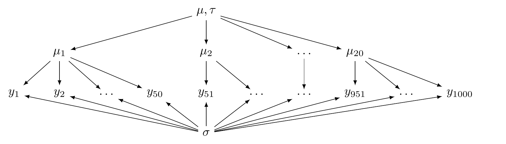
FIGURE 5.1: A directed acyclic graph illustrating a hierarchical model (partial pooling).
There are two other configurations possible that do not involve this hierarchical structure and which represent two alternative, extreme scenarios.
One of these two configurations is called the complete pooling model, Here, the data \(y_n\) are assumed to be generated from a single distribution:
\[\begin{equation} y_n \sim \mathit{Normal}(\mu,\sigma). \end{equation}\]
This model is an intercept only regression similar to what we saw in chapter 3.
Generate fake observations in a vector y based on arbitrary true values in R in the following way.
sigma <- 4
mu <- 100
df_cp <- mutate(df, y = rnorm(N, mu, sigma))
df_cp
## # A tibble: 1,000 × 3
## row subj y
## <int> <int> <dbl>
## 1 1 1 99.4
## 2 2 1 99.1
## 3 3 1 104.
## # ℹ 997 more rowsFit it in brms.
fit_cp <- brm(y ~ 1, df_cp,
             prior =
               c(prior(normal(50, 200), class = Intercept),
prior(normal(2, 5), class = sigma)))fit_cp## ...
## Population-Level Effects:
## Estimate Est.Error l-95% CI u-95% CI Rhat Bulk_ESS Tail_ESS
## Intercept 99.98 0.13 99.73 100.23 1.00 3510 2584
##
## Family Specific Parameters:
## Estimate Est.Error l-95% CI u-95% CI Rhat Bulk_ESS Tail_ESS
## sigma 4.04 0.09 3.87 4.23 1.00 3573 2544
##
## ...The configuration of the complete pooling model is illustrated in Figure 5.2.
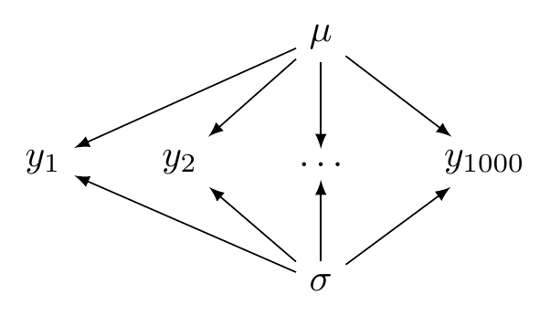
FIGURE 5.2: A directed acyclic graph illustrating a complete pooling model.
The other configuration is called the no pooling model; here, each \(y_n\) is assumed to be generated from an independent distribution:
\[\begin{equation} y_n \sim \mathit{Normal}(\mu_{subj[n]},\sigma) \end{equation}\]
Generate fake observations from the no pooling model in R with arbitrary true values.
sigma <- 4
mu_i <- c(156, 178, 95, 183, 147, 191, 67, 153, 129, 119, 195,
          150, 172, 97, 110, 115, 78, 126, 175, 80)
df_np <- mutate(df, y = rnorm(N, mu_i[subj], sigma))
df_np
## # A tibble: 1,000 × 3
## row subj y
## <int> <int> <dbl>
## 1 1 1 156.
## 2 2 1 162.
## 3 3 1 151.
## # ℹ 997 more rowsFit it in brms. By using the formula 0 + factor(subj), we remove the common intercept and force the model to estimate one intercept for each level of subj. The column subj is converted to a factor so that brms does not interpret it as a number.
fit_np <- brm(y ~ 0 + factor(subj), df_np,
             prior =
               c(prior(normal(0, 200), class = b),
                 prior(normal(2, 5), class = sigma)))
The summary shows now the 20 estimates of \(\mu_i\) as b_factorsubj and \(\sigma\). (We ignore lp__ and lprior.)
fit_np %>% posterior_summary()## Estimate Est.Error Q2.5 Q97.5
## b_factorsubj1 154.70 0.5726 153.57 155.8
## b_factorsubj2 178.49 0.5594 177.41 179.5
## b_factorsubj3 95.53 0.5669 94.41 96.6
## b_factorsubj4 184.39 0.5658 183.28 185.5
## b_factorsubj5 146.70 0.5602 145.60 147.8
## b_factorsubj6 191.54 0.5671 190.40 192.7
## b_factorsubj7 67.60 0.5635 66.52 68.7
## b_factorsubj8 152.70 0.5904 151.54 153.8
## b_factorsubj9 129.34 0.5810 128.24 130.4
## b_factorsubj10 119.70 0.5573 118.59 120.8
## b_factorsubj11 194.94 0.5894 193.81 196.1
## b_factorsubj12 149.71 0.5711 148.61 150.8
## b_factorsubj13 171.77 0.5707 170.68 172.9
## b_factorsubj14 97.03 0.5539 95.96 98.1
## b_factorsubj15 110.48 0.5575 109.38 111.6
## b_factorsubj16 115.41 0.5678 114.32 116.6
## b_factorsubj17 77.87 0.5776 76.75 79.0
## b_factorsubj18 125.50 0.5582 124.41 126.6
## b_factorsubj19 174.75 0.5668 173.66 175.9
## b_factorsubj20 80.13 0.5889 78.98 81.3
## sigma 4.02 0.0903 3.85 4.2
## lprior -131.53 0.0115 -131.55 -131.5
## lp__ -2939.76 3.2261 -2947.05 -2934.5Unlike the hierarchical model, now there is no common distribution that generates the \(\mu_i\) parameters. This is illustrated in Figure 5.3.
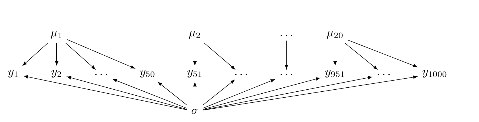
FIGURE 5.3: A directed acyclic graph illustrating a no pooling model.
The hierarchical model lies between these two extremes and for this reason is sometimes called a partial pooling model. One way that the hierarchical model is often described is that the estimates \(\mu_i\) “borrow strength” from the parameter \(\mu\) (which represents the grand mean in the above example).
An important practical consequence of partial pooling is the idea of “borrowing strength from the mean”: if we have very sparse data from a particular member of a group (e.g., missing data from a particular subject), the estimate \(\mu_i\) of that particular group member \(n\) is determined by the parameter \(\mu\). In other words, when the data are sparse for group member \(n\), the posterior estimate \(\mu_i\) is determined largely by the prior \(p(\mu)\). In this sense, even the frequentist hierarchical modeling software in R, lmer from the package lme4, is essentially Bayesian in formulation (except of course that there is no prior as such on \(\mu\)).
So far we focused on the structure of \(\mu\), the location parameter of the likelihood. We could even have partial pooling, complete pooling or no pooling with respect to \(\sigma\), the scale parameter of the likelihood. More generally, any parameter of a likelihood can have any of these kinds of pooling.
In the coming sections, we will be looking at each of these models with more detail and using realistic examples.
Box 5.1 Finitely exchangeable random variables
Formally, we say that the random variables \(Y_1,\dots,Y_N\) are finitely exchangeable if, for any set of particular outcomes of an experiment \(y_1,\dots,y_N\), the probability \(p(y_1,\dots,y_N)\) that we assign to these outcomes is unaffected by permuting the labels given to the variables. In other words, for any permutation \(\pi(n)\), where \(n=1,\dots,N\) ( \(\pi\) is a function that takes as input the positive integer \(n\) and returns another positive integer; e.g., the function takes a subject indexed as 1, and returns index 3), we can reasonably assume that \(p(y_1,\dots,y_N)=p(y_{\pi(1)},\dots,y_{\pi(N)})\). A simple example is a coin tossed twice. Suppose the first coin toss is \(Y_1=1\), a heads, and the second coin toss is \(Y_2=0\), a tails. If we are willing to assume that the probability of getting one heads is unaffected by whether it appears in the first or the second toss, i.e., \(p(Y_1=1,Y_2=0)=p(Y_1=0,Y_2=1)\), then we assume that the indices are exchangeable.
Some important connections and differences between exchangeability and the frequentist concept of independent and identically distributed (iid):
If the data are exchangeable, they are not necessarily iid. For example, suppose you have a box with one black ball and two red balls in it. Your task is to repeatedly draw a ball at random. Suppose that in your first draw, you draw one ball and get the black ball. The probability of getting a black ball in the next two draws is now \(0\). However, if in your first draw you had retrieved a red ball, then there is a non-zero probability of drawing a black ball in the next two draws. The outcome in the first draw affects the probability of subsequent draws–they are not independent. But the sequence of random variables is exchangeable. To see this, consider the following: If a red ball is drawn, count it as a \(0\), and if a black ball is drawn, then count it as \(1\). Then, the three possible outcomes and the probabilities are
- \(1,0,0\); \(P(X_1=1,X_2=0,X_3=0) = \frac{1}{3} \times 1 \times 1=\frac{1}{3}\)
- \(0,1,0\) \(P(X_1=0,X_2=1,X_3=0) = \frac{2}{3} \times \frac{1}{2} \times 1=\frac{1}{3}\)
- \(0,0,1\) \(P(X_1=0,X_2=0,X_3=1) = \frac{2}{3} \times \frac{1}{2} \times 1=\frac{1}{3}\)
The random variables \(X_1,X_2,X_3\) can be permuted and the joint probability distribution (technically, the PMF) is the same in each case.
If the data are exchangeable, then they are identically distributed. For example, in the box containing one black ball and two red balls, suppose we count the draw of a black ball as a \(1\), and the draw of a red ball as a \(0\). Then the probability \(P(X_1=1)=\frac{1}{3}\) and \(P(X_1=0)=\frac{2}{3}\); this is also true for \(X_2\) and \(X_3\). That is, these random variables are identically distributed.
If the data are iid in the standard frequentist sense, then they are exchangeable. For example, suppose you have \(i=1,\dots,n\) instances of a random variable \(X\) whose PDF is \(f(x)\). Suppose also that \(X_i\) are iid. The joint PDF (this can be discrete or continuous, i.e., a PMF or PDF) is
\[\begin{equation} f_{X_1,\dots,X_n}(x_1,\dots,x_n) = f(x_1) \cdot \dots \cdot f(x_n) \end{equation}\]
Because the terms on the right-hand side can be permuted, the labels can be permuted on any of the \(x_i\). This means that \(X_1,\dots,X_n\) are exchangeable.
5.2 A hierarchical model with a normal likelihood: The N400 effect
Event-related potentials (ERPs) allow scientists to observe electrophysiological responses in the brain measured by means of electroencephalography (EEG) that are time-locked to a specific event (i.e., the presentation of the stimuli). A very robust ERP effect in the study of language is the N400. Words with low predictability are accompanied by an N400 effect in comparison with high-predictable words, this is a relative negativity that peaks around 300-500 ms after word onset over central parietal scalp sites (first reported in Kutas and Hillyard 1980, for semantic anomalies, and in 1984 for low predictable word; for a review, see Kutas and Federmeier 2011). The N400 is illustrated in Figure 5.4.

FIGURE 5.4: Typical ERP for the grand average across the N400 spatial window (central parietal electrodes: Cz, CP1, CP2, P3, Pz, P4, POz) for high and low predictability nouns (specifically from the constraining context of the experiment reported in Nicenboim, Vasishth, and Rösler 2020). The x-axis indicates time in seconds and the y-axis indicates voltage in microvolts (unlike many EEG/ERP plots, the negative polarity is plotted downwards).
For example, in (1) below, the continuation ‘paint’ has higher predictability than the continuation ‘dog’, and thus we would expect a more negative signal, that is, an N400 effect, in ‘dog’ in (b) in comparison with ‘paint’ in (a). It is often the case that predictability is measured with a cloze task (see section 1.4).
- Example from Kutas and Hillyard (1984)
- Don’t touch the wet paint.
- Don’t touch the wet dog.
The EEG data are typically recorded in tens of electrodes every couple of milliseconds, but for our purposes (i.e., for learning about Bayesian hierarchical models), we can safely ignore the complexity of the data. A common way to simplify the high-dimensional EEG data when we are dealing with the N400 is to focus on the average amplitude of the EEG signal at the typical spatio-temporal window of the N400 (for example, see Frank et al. 2015).
For this example, we are going to focus on the N400 effect for critical nouns from a subset of the data of Nieuwland et al. (2018). Nieuwland et al. (2018) presented a replication attempt of an original experiment of DeLong, Urbach, and Kutas (2005) with sentences like (2).
- Example from DeLong, Urbach, and Kutas (2005)
- The day was breezy so the boy went outside to fly a kite.
- The day was breezy so the boy went outside to fly an airplane.
We’ll ignore the goal of original experiment (DeLong, Urbach, and Kutas 2005), and its replication (Nieuwland et al. 2018). We are going to focus on the N400 at the final nouns in the experimental stimuli. In example (2), for example, the final noun ‘kite’ has higher predictability than ‘airplane’, and thus we would expect a more negative signal in ‘airplane’ in (b) in comparison with ‘kite’ in (a).
To speed up computation, we restrict the data set of Nieuwland et al. (2018) to the subjects from the Edinburgh lab. This subset of the data can be found in df_eeg in the bcogsci package. Center the cloze probability before using it as a predictor.
data("df_eeg")
(df_eeg <- df_eeg %>%
  mutate(c_cloze = cloze - mean(cloze)))
## # A tibble: 2,863 × 7
## subj cloze item n400 cloze_ans N c_cloze
## <dbl> <dbl> <dbl> <dbl> <dbl> <dbl> <dbl>
## 1 1 0 1 7.08 0 44 -0.476
## 2 1 0.03 2 -0.68 1 44 -0.446
## 3 1 1 3 1.39 44 44 0.524
## # ℹ 2,860 more rows# Number of subjects
df_eeg %>%
distinct(subj) %>%
count()## # A tibble: 1 × 1
## n
## <int>
## 1 37One convenient aspect of using averages of EEG data is that they are roughly normally distributed. This allows us to use the normal likelihood. Figure 5.5 shows the distribution of the data.
df_eeg %>% ggplot(aes(n400)) +
  geom_histogram(binwidth = 4,
                 colour = "gray",
                 alpha = .5,
                 aes(y = after_stat(density))) +
  stat_function(fun = dnorm,
                args = list(mean = mean(df_eeg$n400),
                            sd = sd(df_eeg$n400))) +
  xlab("Average voltage in microvolts for
       the N400 spatiotemporal window")
FIGURE 5.5: Histogram of the N400 averages for every trial, overlaid is a density plot of a normal distribution.
5.2.1 Complete pooling model (\(M_{cp}\))
We’ll start from the simplest model which is basically the linear regression we encountered in the preceding chapter.
5.2.1.1 Model assumptions
This model, call it \(M_{cp}\), makes the following assumptions.
- The EEG averages for the N400 spatiotemporal window are normally distributed.
- Observations are independent.
- There is a linear relationship between cloze and the EEG signal for the trial.
This model is incorrect for these data due to assumption (2) being violated.
With the last assumption, we are saying that the difference in the average signal when we compare nouns with cloze probability of 0 and 0.1 is the same as the difference in the signal when we compare nouns with cloze values of 0.1 and 0.2 (or 0.9 and 1). This is just an assumption, and it may not necessarily be the case in the actual data. This means that we are going to get a posterior for \(\beta\) conditional on the assumption that the linear relationship holds. Even if it approximately holds, we still don’t know how much we deviate from this assumption.
We can now decide on a likelihood and priors.
5.2.1.2 Likelihood and priors
A normal likelihood seems reasonable for these data:
\[\begin{equation} signal_n \sim \mathit{Normal}( \alpha + c\_cloze_n \cdot \beta,\sigma) \tag{5.1} \end{equation}\]
where \(n =1, \ldots, N\), and \(signal\) is the dependent variable (average signal in the N400 spatiotemporal window in microvolts). The variable \(N\) represents the total number of data points.
As always we need to rely on our previous knowledge and domain expertise to decide on priors. We know that ERPs (signals time-locked to a stimulus) have mean amplitudes of a couple of microvolts: This is easy to see in any plot of the EEG literature. This means that we don’t expect the effect of our manipulation to exceed, say, \(10 \mu V\). As before, a priori we’ll assume that effects can be negative or positive. We can quantify our prior knowledge regarding plausible values of \(\beta\) as normally distributed centered at zero with a standard deviation of \(10 \mu V\). (Other values such as \(5 \mu V\) would have been also reasonable, since it would entail that 95% of the prior mass probability is between \(-10\)$ and \(10 \mu V\).)
If the signal for each ERP is baselined, that is, the mean signal of a time window before the time window of interest is subtracted from the time window of interest, then the mean signal would be relatively close to \(0\). Since we know that the ERPs were baselined in this study, we expect that the grand mean of our signal should be relatively close to zero. Our prior for \(\alpha\) is then normally distributed centered in zero with a standard deviation of \(10 \mu V\) as well.
The standard deviation of our signal distribution is harder to guess. We know that EEG signals are quite noisy, and that the standard deviation must be higher than zero. Our prior for \(\sigma\) is a truncated normal distribution with location zero and scale 50. Recall that since we truncate the distribution, the parameters location and scale do not correspond to the mean and standard deviation of the new distribution; see Box 4.1.
We can draw random samples from this truncated distribution and calculate their mean and standard deviation:
samples <- rtnorm(20000, mean = 0, sd = 50, a = 0)
c(mean = mean(samples), sd = sd(samples))
## mean sd
## 39.7 30.0So we are essentially saying that we assume a priori that we will find the true standard deviation of the signal in the following interval with 95% probability:
quantile(samples, probs = c(0.025, .975))## 2.5% 97.5%
## 1.61 111.91# Analytically:
# c(qtnorm(.025, 0, 50, a = 0), qtnorm(.975, 0, 50, a = 0))To sum up, we are going to use the following priors:
\[\begin{equation} \begin{aligned} \alpha &\sim \mathit{Normal}(0,10)\\ \beta &\sim \mathit{Normal}(0,10)\\ \sigma &\sim \mathit{Normal}_{+}(0,50) \end{aligned} \end{equation}\]
A model such as \(M_{cp}\) is sometimes called a fixed-effects model: all the parameters are fixed in the sense that do not vary from subject to subject or from item to item. A similar frequentist model would correspond to fitting a simple linear model using the lm function: lm(n400 ~ 1 + cloze, data = df_eeg).
We fit this model in brms as follows (the default family is gaussian() so we can omit it). As with the lm function in R, by default an intercept is fitted and thus n400 ~ c_cloze is equivalent to n400 ~ 1 + c_cloze:
fit_N400_cp <-
  brm(n400 ~ c_cloze,
      prior = c(prior(normal(0, 10), class = Intercept),
                prior(normal(0, 10), class = b, coef = c_cloze),
                prior(normal(0, 50), class = sigma)),
      data = df_eeg)
For now, check the summary, and plot the posteriors of the model (Figure 5.6).
fit_N400_cp## ...
## Population-Level Effects:
## Estimate Est.Error l-95% CI u-95% CI Rhat Bulk_ESS Tail_ESS
## Intercept 3.66 0.22 3.22 4.09 1.00 3991 2906
## c_cloze 2.27 0.55 1.22 3.37 1.00 3841 2588
##
## Family Specific Parameters:
## Estimate Est.Error l-95% CI u-95% CI Rhat Bulk_ESS Tail_ESS
## sigma 11.82 0.16 11.51 12.14 1.00 4389 3109
##
## ...plot(fit_N400_cp)
FIGURE 5.6: Posterior distributions of the complete pooling model, fit_N400_cp.
5.2.2 No pooling model (\(M_{np}\))
One of the assumptions of the previous model is clearly wrong: observations are not independent, they are clustered by subject (and also by the specific item, but we’ll ignore this until section 5.2.4). It is reasonable to assume that EEG signals are more similar within subjects than between them. The following model assumes that each subject is completely independent from each other.18
5.2.2.1 Model assumptions
- EEG averages for the N400 spatio-temporal window are normally distributed.
- Every subject’s model is fit independently of the other subjects; the subjects have no parameters in common (an exception is the standard deviation, \(\sigma\); this is the same for all subjects in Equation (5.2)).
- There is a linear relationship between cloze and the EEG signal for the trial.
What likelihood and priors can we choose here?
5.2.2.2 Likelihood and priors
The likelihood is a normal distribution as before:
\[\begin{equation} signal_n \sim \mathit{Normal}( \alpha_{subj[n]} + c\_cloze_n \cdot \beta_{subj[n]},\sigma) \tag{5.2} \end{equation}\]
As before, \(n\) represents each observation, that is, the \(n\)th row in the data frame, which has \(N\) rows, and now the index \(i\) identifies the subject. The notation \(subj[n]\), which roughly follows Gelman and Hill (2007), identifies the subject index; for example, if \(subj[10]=3\), then the \(10\)th row of the data frame is from subject \(3\).
We define the priors as follows:
\[\begin{equation} \begin{aligned} \alpha_{i} &\sim \mathit{Normal}(0,10)\\ \beta_{i} &\sim \mathit{Normal}(0,10)\\ \sigma &\sim \mathit{Normal}_+(0,50) \end{aligned} \end{equation}\]
In brms, such a model can be fit by removing the common intercept with the formula n400 ~ 0 + factor(subj) + c_cloze:factor(subj).
This formula forces the model to estimate one intercept and one slope for each level of subj.19
The by-subject intercepts are indicated with factor(subj) and the by-subject slopes with c_cloze:factor(subj). It’s very important to specify that subject should be treated as a factor and not as a number; we don’t assume that subject number 3 will show 3 times more positive (or negative) average signal than subject number 1! The model fits 37 independent intercepts and 37 independent slopes. By setting a prior to class = b and omitting coef, we are essentially setting identical priors to all the intercepts and slopes of the model. The parameters are independent from each other; it is only our previous knowledge (or prior beliefs) about their possible values (encoded in the priors) that is identical. We can set different priors to each intercept and slope, but that will mean setting 74 priors!
fit_N400_np <- brm(n400 ~ 0 + factor(subj) + c_cloze:factor(subj),
                   prior = c(prior(normal(0, 10), class = b),
                             prior(normal(0, 50), class = sigma)),
                   data = df_eeg)
For this model, printing a summary means printing the 75 parameters (\(\alpha_{1,...,37}\), \(\beta_{1,...,37}\), and \(\sigma\)). We could do this as always by printing out the model results: just type fit_N400_np.
It may be easier to understand the output of the model by plotting \(\beta_{1,..,37}\) using bayesplot. (brms also includes a wrapper for this function called stanplot.) We can take a look at the internal names that brms gives to the parameters with variables(fit_N400_np); they are b_factorsubj, then the subject index and then :c_cloze. The code below changes the subject labels back to their original numerical indices and plots them in Figure 5.7. The subjects are ordered by the magnitude of their mean effects.
The model \(M_{np}\) does not estimate a unique population-level effect; instead, there is a different effect estimated for each subject. However, given the posterior means from each subject, it is still possible to calculate the average of these estimates \(\hat\beta_{1,...,I}\), where \(I\) is the total number of subjects:
# parameter name of beta by subject:
ind_effects_np <- paste0("b_factorsubj",
                         unique(df_eeg$subj), ":c_cloze")
beta_across_subj <- as.data.frame(fit_N400_np) %>%
  #removes the meta data from the object
  select(all_of(ind_effects_np)) %>%
  rowMeans()

# Calculate the average of these estimates
(grand_av_beta <- tibble(mean = mean(beta_across_subj),
                         lq = quantile(beta_across_subj, c(.025)),
                         hq = quantile(beta_across_subj, c(.975))))
## # A tibble: 1 × 3
## mean lq hq
## <dbl> <dbl> <dbl>
## 1 2.18 1.17 3.20In Figure 5.7, the 95% credible interval of this overall mean effect is plotted as two vertical lines together with the effect of cloze probability for each subject (ordered by effect size). Here, rather than using a plotting function from brms, we can extract the summary of by-subject effects, reorder them by magnitude, and then plot the summary with a custom plot using ggplot2.
# make a table of beta's by subject
beta_by_subj <- posterior_summary(fit_N400_np,
                                  variable = ind_effects_np) %>%
  as.data.frame() %>%
  mutate(subject = 1:n()) %>%
  ## reorder plot by magnitude of mean:
  arrange(Estimate) %>%
  mutate(subject = factor(subject, levels = subject))
The code below generates Figure 5.7.
ggplot(beta_by_subj,
       aes(x = Estimate, xmin = Q2.5, xmax = Q97.5, y = subject)) +
  geom_point() +
  geom_errorbarh() +
  geom_vline(xintercept = grand_av_beta$mean) +
  geom_vline(xintercept = grand_av_beta$lq, linetype = "dashed") +
  geom_vline(xintercept = grand_av_beta$hq, linetype = "dashed") +
  xlab("By-subject effect of cloze probability in microvolts")
FIGURE 5.7: 95% credible intervals of the effect of cloze probability for each subject according to the no pooling model, fit_N400_np. The solid vertical line represents the mean over all the subjects; and the broken vertical lines mark the 95% credible interval for this mean.
5.2.3 Varying intercepts and varying slopes model (\(M_{v}\))
One major problem with the no-pooling model is that we completely ignore the fact that the subjects were doing the same experiment. We fit each subject’s data ignoring the information available in the other subjects’ data. The no-pooling model is very likely to overfit the individual subjects’ data; we are likely to ignore the generalities of the data and we may end up overinterpreting noisy estimates from each subject’s data. The model can be modified to explicitly assume that the subjects have an overall effect common to all the subjects, with the individual subjects deviating from this common effect.
In the model that we fit next, we will assume that there is an overall effect that is common to the subjects and, importantly, that all subjects’ parameters originate from one common (normal) distribution. This model specification will result in the estimation of posteriors for each subject being also influenced by what we know about all the subjects together. We begin with a hierarchical model with uncorrelated varying intercepts and slopes. The analogous frequentist model can be fit using lmer from the package lme4, using (1+c_cloze||subj) or, equivalently, (c_cloze||subj) for the by-subject random effects.
5.2.3.1 Model assumptions
- EEG averages for the N400 spatio-temporal window are normally distributed.
- Each subject deviates to some extent (this is made precise below) from the grand mean and from the mean effect of predictability. This implies that there is some between-subject variability in the individual-level intercept and slope adjustments by subject.
- There is a linear relationship between cloze and the EEG signal.
5.2.3.2 Likelihood and priors
The likelihood now incorporates the assumption that both the intercept and slope are adjusted by subject.
\[\begin{equation} signal_n \sim \mathit{Normal}(\alpha + u_{subj[n],1} + c\_cloze_n \cdot (\beta+ u_{subj[n],2}),\sigma) \end{equation}\]
\[\begin{equation} \begin{aligned} \alpha &\sim \mathit{Normal}(0,10)\\ \beta &\sim \mathit{Normal}(0,10)\\ u_1 &\sim \mathit{Normal}(0,\tau_{u_1})\\ u_2 &\sim \mathit{Normal}(0,\tau_{u_2})\\ \tau_{u_1} &\sim \mathit{Normal}_+(0,20) \\ \tau_{u_2} &\sim \mathit{Normal}_+(0,20) \\ \sigma &\sim \mathit{Normal}_+(0,50) \end{aligned} \end{equation}\]
In this model each subject has their own intercept adjustment, \(u_{subj,1}\), and slope adjustment, \(u_{subj,2}\).20 If \(u_{subj,1}\) is positive, the subject will have a more positive EEG signal than the grand mean average. If \(u_{subj,2}\) is positive, the subject will have a more positive EEG response to a change of one unit in c_cloze than the overall mean effect (i.e., there will be a more positive effect of cloze probability on the N400). The parameters \(u\) are sometimes called random effects and thus a model with fixed effects (\(\alpha\) and \(\beta\)) and random effects is called a mixed model. However, random effects have different meanings in different contexts. To avoid ambiguity, brms calls these random-effects parameters group-level effects. Since we are estimating \(\alpha\) and \(u\) at the same time and we assume that the average of the \(u\)’s is \(0\) (since it is assumed to be normally distributed with mean \(0\)), what is common between the subjects, the grand mean, is estimated as the intercept \(\alpha\), and the deviations of individual subjects’ means from this grand mean are the adjustments \(u_1\). Similarly, the mean effect of cloze is estimated as \(\beta\), and the deviations of individual subjects’ mean effects of cloze from \(\beta\) are the adjustment \(u_2\). The standard deviations of these two adjustment terms, \(\tau_{u_1}\) and \(\tau_{u_2}\), respectively, represent between subject variability; see Box 5.2.
Thus, the model \(M_{v}\) has three standard deviations: \(\sigma\), \(\tau_{u_1}\) and \(\tau_{u_2}\). In statistics, it is conventional to talk about variances (the square of these standard deviations); for this reason, these standard deviations are also (confusingly) called variance components. The variance components \(\tau_{u_1}\) and \(\tau_{u_2}\) characterize between-subject variability, and the variance component \(\sigma\) characterizes within-subject variability.
The by-subject adjustments \(u_1\) and \(u_2\) are parameters in the model, and therefore have priors defined on them. By contrast, in the frequentist lmer model, the adjustments \(u_1\) and \(u_2\) are not parameters; they are called conditional modes; see Bates, Mächler, et al. (2015b).
Parameters that appear in the prior specifications for parameters, such as \(\tau_u\), are often called hyperparameters,21 and the priors on such hyperparameters are called hyperpriors. Thus, the parameter \(u_1\) has \(\mathit{Normal}(0,\tau_{u_1})\) as a prior; \(\tau_{u_1}\) is a hyperparameter, and the hyperprior on \(\tau_{u_1}\) is \(\mathit{Normal}(0,20)\).22
We know that in general, in EEG experiments, the standard deviations for the by-subject adjustments are smaller than the standard deviation of the observations (which is the within-subjects standard deviation). That is, usually the between-subject variability in the intercepts and slopes is smaller than the within-subjects variability in the data. For this reason, reducing the scale of the truncated normal distribution to \(20\) (in comparison to \(50\)) seems reasonable for the priors of the \(\tau\) parameters. As always, we can do a sensitivity analysis to verify that our priors are reasonably uninformative (if we intended them to be uninformative).
Box 5.2 Some important (and sometimes confusing) points:
Why does \(u\) have a mean of \(0\)?
Because we want \(u\) to capture only differences between subjects, we could achieve the same by assuming the following relationship between the likelihood and the intercept and slope:
\[\begin{equation} \begin{aligned} signal_n &\sim \mathit{Normal}(\alpha_{subj[n]} + \beta_{subj[n]} \cdot c\_cloze_n, \sigma) \\ \alpha_i &\sim \mathit{Normal}(\alpha,\tau_{u_1})\\ \beta_i &\sim \mathit{Normal}(\beta,\tau_{u_2})\\ \end{aligned} \end{equation}\]
In fact, this is another common way to write the model.
Why do the adjustments \(u\) have a normal distribution?
Mostly by convention, the adjustments \(u\) are assumed to come from a normal distribution. Another reason is that if we don’t know anything about the distribution besides its mean and variance, the normal distribution is the most conservative assumption (see chapter 9 of McElreath 2020).
For now, we are assuming that there is no relationship (no correlation) between the by-subject intercept and slope adjustments \(u_1\) and \(u_2\); this lack of correlation is indicated in brms using the double pipe ||. The double pipe is also used in the same way in lmer from the package lme4 (in fact brms bases its syntax on that of the lme4 package).
In brms, we need to specify hyperpriors for \(\tau_{u_1}\) and \(\tau_{u_2}\); these are called sd in brms, to distinguish these standard deviations from the standard deviation of the residuals \(\sigma\). As with the population-level effects, the by-subjects intercept adjustments are implicitly fit for the group-level effects and thus (c_cloze || subj) is equivalent to (1 + c_cloze || subj). If we don’t want an intercept we need to explicitly indicate it with (0 + c_cloze || subj) or (-1 + c_cloze || subj). Such a removal of the intercept is not normally done.
prior_v <-
  c(prior(normal(0, 10), class = Intercept),
    prior(normal(0, 10), class = b, coef = c_cloze),
    prior(normal(0, 50), class = sigma),
    prior(normal(0, 20), class = sd, coef = Intercept, group = subj),
    prior(normal(0, 20), class = sd, coef = c_cloze, group = subj))
fit_N400_v <- brm(n400 ~ c_cloze + (c_cloze || subj),
                  prior = prior_v,
                  data = df_eeg)
When we print a brms fit, we first see the summaries of the posteriors of the standard deviation of the by-group intercept and slopes, \(\tau_{u_1}\) and \(\tau_{u_2}\) as sd(Intercept) and sd(c_cloze), and then, as with previous models, the population-level effects, \(\alpha\) and \(\beta\) as Intercept and c_cloze, and the scale of the likelihood, \(\sigma\), as sigma. The full summary can be printed out by typing:
fit_N400_vBecause the above command will result in some pages of output, it is easier to understand the summary graphically (Figure 5.8). Rather than the wrapper plot(), we use the original function of the package bayesplot, mcmc_dens(), to only show density plots. We extract the first 5 parameters of the model with variables(fit_N400_v)[1:5].
mcmc_dens(fit_N400_v, pars = variables(fit_N400_v)[1:5])
FIGURE 5.8: Posterior distributions of the parameters in the model fit_N400_v.
Because we estimated how the population-level effect of cloze is adjusted for each subject, we could examine how each subject is being affected by the manipulation. For this we do the following, and we plot it in Figure 5.9. These are adjustments, \(u_{1,1},u_{1,...},u_{1,37}\), and not the effect of the manipulation by subject, \(\beta + [u_{1,1},u_{1,...},u_{1,37}]\). The code below produces Figure 5.9.
# make a table of u_2s
ind_effects_v <- paste0("r_subj[", unique(df_eeg$subj),
                        ",c_cloze]")
u_2_v <- posterior_summary(fit_N400_v, variable = ind_effects_v) %>%
  as_tibble() %>%
  mutate(subj = 1:n()) %>%
  ## reorder plot by magnitude of mean:
  arrange(Estimate) %>%
  mutate(subj = factor(subj, levels = subj))
# We plot:
ggplot(u_2_v,
       aes(x = Estimate, xmin = Q2.5, xmax = Q97.5, y = subj)) +
  geom_point() +
  geom_errorbarh() +
  xlab("By-subject adjustment to the slope in microvolts")
FIGURE 5.9: 95% credible intervals of adjustments to the effect of cloze probability for each subject (\(u_{1,1..37}\)) according to the varying intercept and varying slopes model, fit_N400_v. To obtain the effect of cloze probability for each subject, we would need to add the estimate of \(\beta\) to each adjustment.
There is an important difference between the no-pooling model and the varying intercepts and slopes model we just fit. The no-pooling model fits each individual subject’s intercept and slope independently for each subject. By contrast, the varying intercepts and slopes model takes all the subjects’ data into account in order to compute the fixed effects \(\alpha\) and \(\beta\); and the model “shrinks” (Pinheiro and Bates 2000) the by-subject intercept and slope adjustments towards the fixed effects estimates. In Figure 5.10, we can see the shrinkage of the estimates in the varying intercepts model by comparing them with the estimates of the no pooling model (\(M_{np}\)).
# Extract parameter estimates from the no pooling model:
par_np <- posterior_summary(fit_N400_np, variable = ind_effects_np) %>%
  as_tibble() %>%
  mutate(model = "No pooling",
         subj = unique(df_eeg$subj))
# For the hierarchical model, the code is more complicated
# because we want the effect (beta) + adjustment.
# Extract the overall group level effect:
beta <- c(as_draws_df(fit_N400_v)$b_c_cloze)
# Extract the individual adjustments:
ind_effects_v <- paste0("r_subj[", unique(df_eeg$subj), ",c_cloze]")
adjustment <- as_draws_matrix(fit_N400_v, variable = ind_effects_v)
# Get the by subject effects in a data frame where each adjustment
# is in each column.
# Remove all the draws meta data by using as.data.frame
by_subj_effect <- as.data.frame(beta + adjustment)
# Summarize them by getting a table with the mean and the
# quantiles for each column and then binding them.
par_h <- lapply(by_subj_effect, function(x) {
  tibble(Estimate = mean(x),
         Q2.5 = quantile(x, .025),
         Q97.5 = quantile(x, .975))}) %>%
  bind_rows() %>%
  # Add a column to identify that the model,
  # and one with the subject labels:
  mutate(model = "Hierarchical",
         subj = unique(df_eeg$subj))
# The mean and 95% CI of both models in one data frame:
by_subj_df <- bind_rows(par_h, par_np) %>%
  arrange(Estimate) %>%
  mutate(subj = factor(subj, levels = unique(.data$subj)))
b_c_cloze <- posterior_summary(fit_N400_v, variable = "b_c_cloze")
ggplot(by_subj_df,
aes(ymin = Q2.5, ymax = Q97.5, x = subj,
y = Estimate, color = model, shape = model)) +
geom_errorbar(position = position_dodge(1)) +
geom_point(position = position_dodge(1)) +
# We'll also add the mean and 95% CrI of the overall difference
# to the plot:
geom_hline(yintercept = b_c_cloze[, "Estimate"]) +
geom_hline(yintercept = b_c_cloze[, "Q2.5"],
linetype = "dotted", linewidth = .5) +
geom_hline(yintercept = b_c_cloze[, "Q97.5"],
linetype = "dotted", linewidth = .5) +
xlab("N400 effect of predictability") +
coord_flip()
FIGURE 5.10: This plot compares the estimates of the effect of cloze probability for each subject between (i) the no pooling, fit_N400_np and (ii) the varying intercepts and varying slopes, hierarchical, model, fit_N400_v.
5.2.4 Correlated varying intercept varying slopes model (\(M_{h}\))
The model \(M_{v}\) allowed for differences in intercepts (mean voltage) and slopes (effects of cloze) across subjects, but it has the implicit assumption that these varying intercepts and varying slopes are independent. It is in principle possible that subjects showing more negative voltage may also show stronger effects (or weaker effects). Next, we fit a model that allows a correlation between the intercepts and slopes. We model the correlation between varying intercepts and slopes by defining a variance-covariance matrix \(\boldsymbol{\Sigma}\) between the by-subject varying intercepts and slopes, and by assuming that both adjustments (intercept and slope) come from a multivariate (in this case, a bivariate) normal distribution.
- In \(M_h\), we model the EEG data with the following assumptions:
- EEG averages for the N400 spatio-temporal window are normally distributed.
- Some aspects of the mean signal voltage and of the effect of predictability depend on the subject, and these two might be correlated, i.e., we assume group-level intercepts and slopes, and allow a correlation between them by-subject.
- There is a linear relationship between cloze and the EEG signal for the trial.
The likelihood remains identical to the model \(M_v\), which assumes no correlation between group-level intercepts and slopes (section 5.2.3):
\[\begin{equation} signal_n \sim \mathit{Normal}(\alpha + u_{subj[n],1} + c\_cloze_n \cdot (\beta + u_{subj[n],2}),\sigma) \end{equation}\]
The correlation is indicated in the priors on the adjustments for intercept \(u_{1}\) and slopes \(u_{2}\).
- Priors: \[\begin{equation} \begin{aligned} \alpha & \sim \mathit{Normal}(0,10) \\ \beta & \sim \mathit{Normal}(0,10) \\ \sigma &\sim \mathit{Normal}_+(0,50)\\ {\begin{pmatrix} u_{i,1} \\ u_{i,2} \end{pmatrix}} &\sim {\mathcal {N}} \left( {\begin{pmatrix} 0\\ 0 \end{pmatrix}} ,\boldsymbol{\Sigma_u} \right) \end{aligned} \end{equation}\]
In this model, a bivariate normal distribution generates the varying intercepts and varying slopes \(\mathbf{u}\); this is an \(n\times 2\) matrix. The variance-covariance matrix \(\boldsymbol{\Sigma_u}\) defines the standard deviations of the varying intercepts and varying slopes, and the correlation between them. Recall from section 1.6.2 that the diagonals of the variance-covariance matrix contain the variances of the correlated random variables, and the off-diagonals contain the covariances. In this example, the covariance \(Cov(u_1,u_2)\) between two variables \(u_1\) and \(u_2\) is defined as the product of their correlation \(\rho\) and their standard deviations \(\tau_{u_1}\) and \(\tau_{u_2}\). In other words, \(Cov(u_1,u_2) = \rho_u \tau_{u_1} \tau_{u_2}\).
\[\begin{equation} \boldsymbol{\Sigma_u} = {\begin{pmatrix} \tau_{u_1}^2 & \rho_u \tau_{u_1} \tau_{u_2} \\ \rho_u \tau_{u_1} \tau_{u_2} & \tau_{u_2}^2 \end{pmatrix}} \end{equation}\]
In order to specify a prior for \(\Sigma_u\), we need priors for the standard deviations, \(\tau_{u_1}\), and \(\tau_{u_2}\), and also for their correlation, \(\rho_u\). We can use the same priors for \(\tau\) as before. For the correlation parameter \(\rho_u\) (and the correlation matrix more generally), we use the LKJ prior. The basic idea of the LKJ prior on the correlation matrix is that as its parameter, \(\eta\) (eta), increases, it will favor correlations closer to zero.23 At \(\eta = 1\), the LKJ correlation distribution is uninformative (similar to \(Beta(1,1)\)), at \(\eta < 1\), it favors extreme correlations (similar to \(Beta(a<1,b<1)\)). We set \(\eta = 2\) so that we don’t favor extreme correlations, and we still represent our lack of knowledge through the wide spread of the prior between \(-1\) and \(1\). Thus, \(\eta = 2\) gives us a regularizing, relatively uninformative or mildly informative prior.
Figure 5.11 shows a visualization of different parameterizations of the LKJ prior.


FIGURE 5.11: Visualization of the LKJ correlation distribution prior with four different values of the \(\eta\) parameter.
\[\begin{equation} \begin{aligned} \tau_{u_1} &\sim \mathit{Normal}_+(0,20)\\ \tau_{u_2} &\sim \mathit{Normal}_+(0,20)\\ \rho_u &\sim \mathit{LKJcorr}(2) \end{aligned} \end{equation}\]
In our brms model, we allow a correlation between the by-subject intercepts and slopes by using a single pipe | instead of the double pipe || that we used previously. This convention follows that in the frequentist lmer function. As before, the varying intercepts are implicitly fit.
Because we have a new parameter, the correlation \(\rho_{u}\), we need to add a new prior for this correlation; in brms, this is achieved by addition a prior for the parameter type cor.
prior_h <- c(prior(normal(0, 10), class = Intercept),
             prior(normal(0, 10), class = b, coef = c_cloze),
             prior(normal(0, 50), class = sigma),
             prior(normal(0, 20),
                   class = sd, coef = Intercept,
                   group = subj
                   ),
             prior(normal(0, 20),
                   class = sd, coef = c_cloze,
                   group = subj),
             prior(lkj(2), class = cor, group = subj))
fit_N400_h <- brm(n400 ~ c_cloze + (c_cloze | subj),
                  prior = prior_h,
                  data = df_eeg)
The estimates do not change much in comparison with the varying intercept/slope model, probably because the estimation of the correlation is quite poor (i.e., there is a lot of uncertainty). While the inclusion of the correlation parameter is justified, this results, in our experience, in a slower convergence of the models (see also the discussion at the end of the section 5.2.6).
As before, the estimates are shown graphically, in Figure 5.12. One can access the complete summary as always with fit_N400_h.
plot(fit_N400_h, N = 6)
FIGURE 5.12: The posteriors of the parameters in the model fit_N400_h.
We are now half-way to what is sometimes called the “maximal” hierarchical model (Barr et al. 2013). This usually refers to a model with all the by-participant and by-items group-level variance components allowed by the experimental design and a full variance covariance matrix for all the group-level parameters. Not all variance components are allowed by the experimental design: in particular, between-group manipulations cannot have variance components. For example, even if we assume that the working memory capacity of the subjects might affect the N400, we cannot measure how working memory affects the subjects differently.
When we refer to a full variance-covariance matrix, we mean a variance-covariance matrix where all the elements (variances and covariances) are non-zero. In our previous model, for example, the variance-covariance matrix \(\boldsymbol{\Sigma_u}\) was full because no element was zero. If we assume no correlation between group-level intercept and slope, it would mean to have zeros in the diagonal of the matrix and this would render the model to be identical to \(M_{v}\) defined in section 5.2.3; if we assume that also the bottom right element (\(\tau^2\)) is zero, the model would turn into a varying intercept model (in brms formula n400 ~ c_cloze + (1 | subj)); and if we assume that the matrix has only zeros, the model would turn into a complete pooling model, \(M_{cp}\), as defined in section 5.2.1.
As we will see in section 5.2.6 and in chapter 7, “maximal” is a misnomer for Bayesian models, since this mostly refers to limitations of the popular frequentist package for fitting models, lme4.
The next section spells out a model with full variance-covariance matrix for both subjects and items-level effects.
5.2.5 By-subjects and by-items correlated varying intercept varying slopes model (\(M_{sih}\))
Our new model, \(M_{sih}\) will allow for differences in intercepts (mean voltage) and slopes (effects of predictability) across subjects and across items. In typical Latin square designs, subjects and items are said to be crossed random effects—each subject sees exactly one instance of each item. Here we assume a possible correlation between varying intercepts and slopes by subjects, and another one by items.
- In \(M_{sih}\), we model the EEG data with the following assumptions:
EEG averages for the N400 spatio-temporal window are normally distributed.
Some aspects of the mean signal voltage and of the effect of predictability depend on the subject, i.e., we assume group-level intercepts, and slopes, and a correlation between them by-subject.
Some aspects of the mean signal voltage and of the effect of predictability depend on the item, i.e., we assume group-level intercepts, and slopes, and a correlation between them by-item.
There is a linear relationship between cloze and the EEG signal for the trial.
- Likelihood:
\[\begin{multline} signal_n \sim \mathit{Normal}(\alpha + u_{subj[n],1} + w_{item[n],1} + \\ c\_cloze_n \cdot (\beta + u_{subj[n],2}+ w_{item[n],2}), \sigma) \end{multline}\]
- Priors: \[\begin{equation} \begin{aligned} \alpha & \sim \mathit{Normal}(0,10) \\ \beta & \sim \mathit{Normal}(0,10) \\ \sigma &\sim \mathit{Normal}_+(0,50)\\ {\begin{pmatrix} u_{i,1} \\ u_{i,2} \end{pmatrix}} &\sim {\mathcal {N}} \left( {\begin{pmatrix} 0\\ 0 \end{pmatrix}} ,\boldsymbol{\Sigma_u} \right) \\ {\begin{pmatrix} w_{j,1} \\ w_{j,2} \end{pmatrix}} &\sim {\mathcal {N}} \left( {\begin{pmatrix} 0\\ 0 \end{pmatrix}} ,\boldsymbol{\Sigma_w} \right) \end{aligned} \end{equation}\]
We have added the index \(j\), which represents each item, as we did with subjects; \(item[n]\) indicates the item that corresponds to the observation in the \(n\)-th row of the data frame.
We have hyperparameters and hyperpriors as before:
\[\begin{equation} \begin{aligned} \boldsymbol{\Sigma_u} & = {\begin{pmatrix} \tau_{u_1}^2 & \rho_u \tau_{u_1} \tau_{u_2} \\ \rho_u \tau_{u_1} \tau_{u_2} & \tau_{u_2}^2 \end{pmatrix}}\\ \boldsymbol{\Sigma_w} & = {\begin{pmatrix} \tau_{w_1}^2 & \rho_w \tau_{w_1} \tau_{w_2} \\ \rho_w \tau_{w_1} \tau_{w_2} & \tau_{w_2}^2 \end{pmatrix}} \end{aligned} \end{equation}\]
\[\begin{equation} \begin{aligned} \tau_{u_1} &\sim \mathit{Normal}_+(0,20)\\ \tau_{u_2} &\sim \mathit{Normal}_+(0,20)\\ \rho_u &\sim \mathit{LKJcorr}(2) \\ \tau_{w_1} &\sim \mathit{Normal}_+(0,20)\\ \tau_{w_2} &\sim \mathit{Normal}_+(0,20)\\ \rho_w &\sim \mathit{LKJcorr}(2) \\ \end{aligned} \end{equation}\]
We set identical priors for by-items group-level effects as for by-subject group-level effects, but this only because we don’t have any differentiated prior information about subject-level vs. item-level variation. However, bear in mind that the estimation for items is completely independent from the estimation for subjects. Although we wrote many more equations than before, the brms model is quite straightforward to extend:
prior_sih_full <-
  c(prior(normal(0, 10), class = Intercept),
    prior(normal(0, 10), class = b, coef = c_cloze),
    prior(normal(0, 50), class = sigma),
    prior(normal(0, 20),
          class = sd, coef = Intercept,
          group = subj),
    prior(normal(0, 20),
          class = sd, coef = c_cloze,
          group = subj),
    prior(lkj(2), class = cor, group = subj),
    prior(normal(0, 20),
          class = sd, coef = Intercept,
          group = item),
    prior(normal(0, 20),
          class = sd, coef = c_cloze,
          group = item),
    prior(lkj(2), class = cor, group = item))
fit_N400_sih <- brm(n400 ~ c_cloze + (c_cloze | subj) +
                      (c_cloze | item),
                    prior = prior_sih_full,
                    data = df_eeg)
We can also simplify the call to brms, when we assign the same priors to the by-subject and by-item parameters:
prior_sih <-
  c(prior(normal(0, 10), class = Intercept),
    prior(normal(0, 10), class = b),
    prior(normal(0, 50), class = sigma),
    prior(normal(0, 20), class = sd),
    prior(lkj(2), class = cor))
fit_N400_sih <- brm(n400 ~ c_cloze + (c_cloze | subj) +
                      (c_cloze | item),
                    prior = prior_sih,
                    data = df_eeg)
We have new group-level effects in the summary, but again the estimate of the effect of cloze remains virtually unchanged (Figure 5.13).
fit_N400_sihplot(fit_N400_sih, N = 9)
FIGURE 5.13: The posterior distributions of the parameters in the model fit_N400_sih.
5.2.6 Beyond the maximal model–Distributional regression models
We can use posterior predictive checks to verify that our last model can capture the entire signal distribution. This is shown in Figure 5.14.
pp_check(fit_N400_sih, ndraws = 50, type = "dens_overlay")
FIGURE 5.14: Overlay of densities from the posterior predictive distributions of the model fit_N400_sih.
However, we know that in ERP studies, large levels of impedance between the recording electrodes and the skin tissue increase the noise in the recordings (Picton et al. 2000). Given that skin tissue is different between subjects, it could be the case that the level of noise varies by subject. It might be a good idea to verify that our model is good enough for capturing the by-subject variability. The code below produces Figure 5.15.
pp_check(fit_N400_sih,
          type = "dens_overlay_grouped",
          ndraws = 100,
          group = "subj") +
  xlab("Signal in the N400 spatiotemporal window") +
  theme(legend.position = c(.5,.08))
## Warning: A numeric `legend.position` argument in
## `theme()` was deprecated in ggplot2 3.5.0. ℹ Please
## use the `legend.position.inside` argument of `theme()`
## instead. This warning is displayed once every 8 hours.
## Call `lifecycle::last_lifecycle_warnings()` to see where
## this warning was generated. 
FIGURE 5.15: The plot shows 100 predicted distributions with the label \(y_{rep}\) and the distribution of the average signal data with the label \(y\) density plots for the 37 subjects that participated in the experiment.
Figure 5.15 hints that we might be misfitting some subjects: Some of the by-subject observed distributions of the EEG signal averages look much tighter than their corresponding posterior predictive distributions (e.g., subjects 3, 5, 9, 10, 14), whereas some other by-subject observed distributions look wider (e.g., subjects 25, 26, 27). Another approach to examine whether we misfit the by-subject noise level is to plot posterior distributions of the standard deviations and compare them with the observed standard deviation. This is achieved in the following code, which groups the data by subject, and shows the distribution of standard deviations. The result is shown in Figure 5.16. It is clear now that, for some subjects, the observed standard deviation lies outside the distribution of predictive standard deviations.
pp_check(fit_N400_sih,
         type = "stat_grouped",
         ndraws = 1000,
         group = "subj",
         stat = "sd",
         facet_args = list(scales = "fixed")) +
  scale_x_continuous(breaks = c(8, 12, 16), limits = c(7,19)) +
  theme(legend.position = c(.5,.08))
FIGURE 5.16: Distribution of posterior predicted standard deviations in gray and observed standard deviation in black lines by subject.
Why is our “maximal” hierarchical model misfitting the by-subject distribution of data? This is because, the maximal models are, in general and implicitly, models with the maximal group-level effect structure for the location parameter (e.g., the mean, \(\mu\), in a normal model). Other parameters (e.g., scale or shape parameters) are estimated as auxiliary parameters, and are assumed to be constant across observations and clusters. This assumption is so common that researchers may not be aware that it is just an assumption. In the Bayesian framework, it is easy to change such default assumptions if necessary. Changing the assumption that all subjects have the same residual standard deviation leads to the distributional regression model. Such models can be fit in brms ; see also the brms vignette, https://cran.r-project.org/web/packages/brms/vignettes/brms_distreg.html.
We are going to change our previous likelihood, so that the scale, \(\sigma\) has also a group-level effect structure. We exponentiate \(\sigma\) to make sure that the negative adjustments do not cause \(\sigma\) to become negative.
\[\begin{equation} \begin{aligned} signal_n &\sim \mathit{Normal}(\alpha + u_{subj[n],1} + w_{item[n],1} + \\ & \hspace{2cm} c\_cloze_n \cdot (\beta + u_{subj[n],2}+ w_{item[n],2}), \sigma_n)\\ \sigma_n &= \exp(\sigma_\alpha + \sigma_{u_{subj[n]}}) \end{aligned} \end{equation}\]
We just need to add priors to our new parameters (that replace the old prior for \(\sigma\)). We set the prior to the intercept of the standard deviation, \(\sigma_\alpha\), to be similar to our previous \(\sigma\). For the variance component of \(\sigma\), \(\tau_{\sigma_u}\), we set rather uninformative hyperpriors. Recall that everything is exponentiated when it goes inside the likelihood; that is why we use \(\log(50)\) rather than 50 in \(\sigma\).
\[\begin{equation} \begin{aligned} \sigma_\alpha &\sim \mathit{Normal}(0,log(50))\\ \sigma_u &\sim \mathit{Normal}(0, \tau_{\sigma_u}) \\ \tau_{\sigma_u} &\sim \mathit{Normal}_+(0, 5) \end{aligned} \end{equation}\]
This model can be fit in brms using the internal function brmsformula() (or its shorter alias bf). This is a powerful function that extends the formulas that we used so far allowing for setting a hierarchical regression to any parameter of a model. This will allow us to set a by-subject hierarchical structure to the parameter \(\sigma\). We also need to set new priors; these priors are identified by dpar = sigma.
prior_s <-
  c(prior(normal(0, 10), class = Intercept),
    prior(normal(0, 10), class = b),
    prior(normal(0, 20), class = sd),
    prior(lkj(2), class = cor),
    prior(normal(0, log(50)), class = Intercept, dpar = sigma),
    prior(normal(0, 5),
          class = sd, group = subj,
          dpar = sigma))
fit_N400_s <- brm(brmsformula(
  n400 ~ c_cloze + (c_cloze | subj) + (c_cloze | item),
  sigma ~ 1 + (1 | subj)),
  prior = prior_s, data = df_eeg)
Inspect the output below; notice that our estimate for the effect of cloze
remains very similar to that of the model fit_N400_sih.
Compare the two models’ estimates:
posterior_summary(fit_N400_sih, variable = "b_c_cloze")## Estimate Est.Error Q2.5 Q97.5
## b_c_cloze 2.3 0.694 0.913 3.63posterior_summary(fit_N400_s, variable = "b_c_cloze")## Estimate Est.Error Q2.5 Q97.5
## b_c_cloze 2.28 0.65 0.99 3.59Nonetheless, Figure 5.17 shows that the fit of the model with respect to the by-subject variability is much better than before. Furthermore, Figure 5.18 shows that the observed standard deviations for each subject are well inside the posterior predictive distributions. The code below produces Figure 5.17.
pp_check(fit_N400_s,
          type = "dens_overlay_grouped",
          ndraws = 100,
          group = "subj") +
  xlab("Signal in the N400 spatiotemporal window") +
  theme(legend.position = c(.5,.08))
FIGURE 5.17: The gray density plots show 100 predicted distributions from a model that includes a hierarchical structure for \(\sigma\). The black density plots show the distribution of the average signal data for the 37 subjects in the experiment.

FIGURE 5.18: The gray lines show the distributions of posterior predicted standard deviations from a model that includes a hierarchical structure for \(\sigma\), and observed mean standard deviations by subject (black vertical lines).
The model fit_N400_s raises the question: how much structure should we add to our statistical model? Should we also assume that \(\sigma\) can vary by items, and also by our experimental manipulation? Should we also have a maximal model for \(\sigma\)? Unfortunately, there are no clear answers that apply to every situation. The amount of complexity that we can introduce in a statistical model depends on (i) the answers we are looking for (we should include parameters that represent what we want to estimate), (ii) the size of the data at hand (more complex models require more data), (iii) our computing power (as the complexity increases models take increasingly long to converge and require more computer power to finish the computations in a feasible time frame), and (iv) our domain knowledge.
Whether certain effects should be included in a model also depends on whether they are known to impact posterior inference or statistical testing (e.g., via Bayes factors). For example, it is well known that estimating group-level effects for the location parameter can have a strong influence on the test statistics for the corresponding population-level effect (Barr et al. 2013; Schad, Nicenboim, Bürkner, Betancourt, et al. 2022b). Given that population-level effects are often what researchers care about, it is therefore important to consider group-level effects for the location parameter. However, to our knowledge, it is not clear whether estimating group-level effects for the standard deviation of the likelihood has an impact on inferences for the fixed effects. Maybe there is one, but it is not widely known–statistical research would have to be conducted via simulations to assess whether such an influence can take place. The point here is that for some effects, it’s crucial to include them in the model, because they are known to affect the inferences that we want to draw from the data. Other model components may (presumably) be less decisive. Which ones these are remains an open question for research.
Ultimately, all models are approximations (that’s in the best case; often, they are plainly wrong) and we need to think carefully about which aspects of our data we have to account and which aspects we can abstract away from.
In the context of cognitive modeling, McClelland (2009) argues that models should not focus on a every single detail of the process they intend to explain. In order to understand a model, it needs to be simple enough. However, McClelland (2009) warns us that one must bear in mind that oversimplification does have an impact on what we can conclude from our analysis: A simplification can limit the phenomena that a model addresses, or can even lead to incorrect predictions. There is a continuum between purely statistical models (e.g., a linear regression) and computational cognitive models. For example, we can define “hybrid” models such as the linear ballistic accumulator (Brown and Heathcote 2008; and see Nicenboim 2018 for an implementation in Stan), where a great deal of cognitive detail is sacrificed for tractability. The conclusions of McClelland (2009) apply to any type of model in cognitive science: “Simplification is essential, but it comes at a cost, and real understanding depends in part on understanding the effects of the simplification”.
5.3 A hierarchical log-normal model: The Stroop effect
Next, using data from Ebersole et al. (2016), we illustrate some of the issues that arise with a log-normal likelihood in a hierarchical model. The data are from a Stroop task (Stroop 1935; for a review, see MacLeod 1991). We will analyze a subset of the data of 3337 subjects that participated in one variant of the Stroop task; this was part of a battery of tasks run in Ebersole et al. (2016).
For this variant of the Stroop task, subjects were presented with one word at the center of the screen (“red”, “blue”, or “green”). The word was written in either red, blue, or green color. In one third of the trials, the word matched the color of the text (“congruent” condition); and in the rest of the trials it did not match (“incongruent” condition). Subjects were instructed to only pay attention to the color that the word was written in, and press 1 if the color was red, 2 if it was blue, and 3 if it was green. In the incongruent condition, it is difficult to identify the color when it mismatches the word that is written on the screen. For example, it is hard to respond that the color is blue if the word written on the screen is green but the color it is presented in is blue; naming the color blue here is difficult in comparison to a baseline condition (the congruent condition), in which the word green appears in the color green. This increased difficulty in the incongruent condition is called the Stroop effect; the effect is extremely robust across variations in the task.
This task yields two measures: the accuracy of the decision made, and the time it took to respond. For the Stroop task, accuracy is usually almost at ceiling; to simplify the model, we will ignore accuracy. For a cognitive model that incorporates accuracy and response times into a model to analyze these Stroop data, see Nicenboim (2018).
5.3.1 A correlated varying intercept varying slopes log-normal model
If our theory only focuses on the difference between the response times for the “congruent” vs. “incongruent” condition, we can ignore the actual color presented and the word that was written. We can simply focus on whether a trial was congruent or incongruent. Define a predictor c_cond to represent these two conditions. For simplicity, we will also assume that all subjects share the same variance (as we saw in section 5.2.6, changing this assumption leads to distributional regression models).
The above assumptions mean that we are going to fit the data with the following likelihood. The likelihood function is identical to the one that we fit in section 5.2.4, except that here the location and scale are embedded in a log-normal likelihood rather than a normal likelihood. Equation (5.3) states that we are dealing with a hierarchical model with by-subjects varying intercepts and varying slopes model:
\[\begin{equation} rt_n \sim \mathit{LogNormal}(\alpha + u_{subj[n],1} + c\_cond_n \cdot (\beta + u_{subj[n],2}), \sigma) \tag{5.3} \end{equation}\]
In chapter 8, we will discuss the sum-contrast coding of the two conditions (c_cond). For now, it suffices to say that we assign a +1 to c_cond for the “incongruent” condition, and a -1 for the “congruent” condition (i.e., a sum-contrast coding). Under this contrast coding, if the posterior mean of the parameter \(\beta\) turns out to be positive, that would mean that the model predicts that the incongruent condition has slower reaction times than the congruent one. This is because on average the location of the log-normal likelihood for each condition will be as follows. In Equation (5.4), \(\mu_{incongruent}\) refers to the location of the incongruent condition, and \(\mu_{congruent}\) to the location of the congruent condition.
\[\begin{equation} \begin{aligned} \mu_{incongruent} &= \alpha + 1 \cdot \beta \\ \mu_{congruent} &= \alpha + -1 \cdot \beta \end{aligned} \tag{5.4} \end{equation}\]
We could have chosen to do the opposite contrast coding assignments: \(-1\) for the incongruent condition, and \(+1\) for congruent condition. In that case, if the posterior mean of the parameter \(\beta\) turns out to be positive, that would mean that the incongruent condition has a faster reaction time than the congruent condition. Given that the Stroop effect is very robust, we do not expect such an outcome. In order to make the \(\beta\) parameter easier to interpret, we have chosen the contrast coding where a positive sign on the mean of \(\beta\) implies that the inconguent condition has slower reaction times.
As always, we need priors for all the parameters in our model. For the population-level parameters (or fixed effects), we use the same priors as we did when we were fitting a regression with a log-normal likelihood in section 3.7.2.
\[\begin{equation} \begin{aligned} \alpha & \sim \mathit{Normal}(6, 1.5) \\ \beta & \sim \mathit{Normal}(0, 0.01) \\ \sigma &\sim \mathit{Normal}_+(0, 1) \end{aligned} \end{equation}\]
Here, \(\beta\) represents, on the log scale, the change in the intercept \(\alpha\) as a function of the experimental manipulation. In this model, \(\beta\) will probably be larger in magnitude than for the model that examined the difference in pressing the spacebar for two consecutive trials in section 3.7.2. We might need to examine the prior for \(\beta\) with predictive distributions, but we will delay this for now.
In contrast to our previous models, the intercept \(\alpha\) is not the grand mean of the location. This is because the conditions were not balanced in the experiment (one-third of the conditions were congruent and two-thirds incongruent). The intercept could be interpreted here as the time (in log-scale) it takes to respond if we ignore the experimental manipulation. Next, we turn our attention to the prior specification for the group-level parameters (or random effects). If we assume a possible correlation between by-subject intercepts and slopes, our model will have the following structure. In particular, we have to define priors for the parameters in the variance-covariance matrix \(\Sigma_u\).
\[\begin{equation} \begin{aligned} {\begin{pmatrix} u_{i,1} \\ u_{i,2} \end{pmatrix}} &\sim {\mathcal {N}} \left( {\begin{pmatrix} 0\\ 0 \end{pmatrix}} ,\boldsymbol{\Sigma_u} \right) \end{aligned} \end{equation}\]
\[\begin{equation} \begin{aligned} \boldsymbol{\Sigma_u} & = {\begin{pmatrix} \tau_{u_1}^2 & \rho_u \tau_{u_1} \tau_{u_2} \\ \rho_u \tau_{u_1} \tau_{u_2} & \tau_{u_2}^2 \end{pmatrix}} \end{aligned} \end{equation}\]
In practice, this means that we need priors for the by-subject standard deviations and correlations. For the variance components, we will set a similar prior as for \(\sigma\). We don’t expect the by-group adjustments to the intercept and slope to have more variance than the within-subject variance, so this prior will be quite conservative because it allows for a large range of prior uncertainty. We assign the same prior for the correlations as we did in section 5.2.5.
\[\begin{equation} \begin{aligned} \tau_{u_1} &\sim \mathit{Normal}_+(0,1)\\ \tau_{u_2} &\sim \mathit{Normal}_+(0,1)\\ \rho_u &\sim \mathit{LKJcorr}(2) \end{aligned} \end{equation}\]
We are now ready to fit the model. To speed up computation, we subset 50 subjects of the original data set; both the subsetted data and the original data set can be found in the package bcogsci. If we were analyzing these data for publication in a journal article or the like, we would obviously not subset the data.
We restrict ourselves to the correct trials only, and add a c_cond predictor, sum-coded as described earlier.
data("df_stroop")
(df_stroop <- df_stroop %>%
  mutate(c_cond = if_else(condition == "Incongruent", 1, -1)))
## # A tibble: 3,058 × 5
## subj trial condition RT c_cond
## <dbl> <int> <chr> <int> <dbl>
## 1 1 0 Congruent 1484 -1
## 2 1 1 Incongruent 1316 1
## 3 1 2 Incongruent 628 1
## # ℹ 3,055 more rowsFit the model.
fit_stroop <- brm(RT ~ c_cond + (c_cond | subj),
                  family = lognormal(),
                  prior =
                    c(prior(normal(6, 1.5), class = Intercept),
                      prior(normal(0, .01), class = b),
                      prior(normal(0, 1), class = sigma),
                      prior(normal(0, 1), class = sd),
                      prior(lkj(2), class = cor)),
                  data = df_stroop)
We will focus on \(\beta\) (but you can verify that there is nothing surprising in the other parameters in the model fit_stroop ).
posterior_summary(fit_stroop, variable = "b_c_cond")## Estimate Est.Error Q2.5 Q97.5
## b_c_cond 0.0269 0.00555 0.0159 0.0374As shown in Figure 5.19, if we overlay the density plots for the prior and posterior distributions of \(\beta\), it becomes evident that the prior might have been too restrictive: the posterior is relatively far from the prior, and the prior strongly down-weights the values that the posterior is centered around. Such a strong discrepancy between the prior and posterior can be investigated with a sensitivity analysis.
sample_b_post <- as_draws_df(fit_stroop)$b_c_cond
# We generate samples from the prior as well:
N <- length(sample_b_post)
sample_b_prior <- rnorm(N, 0, .01)
samples <-
  tibble(sample = c(sample_b_post, sample_b_prior),
         distribution = c(rep("posterior", N), rep("prior", N)))
ggplot(samples, aes(x = sample, fill = distribution)) +
  geom_density(alpha = .5)
FIGURE 5.19: The discrepancy between the prior and the posterior distributions for the slope parameter in the model fit_stroop.
5.3.1.1 Sensitivity analysis
Here, the discrepancy evident in Figure 5.19 is investigated with a sensitivity analysis. We will examine what happens for the following priors for \(\beta\). In the models we fit below, all the other parameters have the same priors as in the model fit_stroop; we vary only the priors for \(\beta\).
The different priors are:
- \(\beta \sim \mathit{Normal}(0,0.05)\)
- \(\beta \sim \mathit{Normal}(0,0.1)\)
- \(\beta \sim \mathit{Normal}(0,1)\)
- \(\beta \sim \mathit{Normal}(0,2)\)
We can summarize the estimates of \(\beta\) given different priors as shown in Table 5.1.
| prior | Estimate | Q2.5 | Q97.5 |
|---|---|---|---|
| \(\mathit{Normal}(0, 0.001)\) | \(0.001\) | \(-0.001\) | \(0.003\) |
| \(\mathit{Normal}(0, 0.01)\) | \(0.027\) | \(0.016\) | \(0.037\) |
| \(\mathit{Normal}(0, 0.05)\) | \(0.037\) | \(0.025\) | \(0.049\) |
| \(\mathit{Normal}(0, 0.1)\) | \(0.037\) | \(0.025\) | \(0.049\) |
| \(\mathit{Normal}(0, 1)\) | \(0.038\) | \(0.025\) | \(0.050\) |
| \(\mathit{Normal}(0, 2)\) | \(0.038\) | \(0.026\) | \(0.050\) |
It might be easier to see how much the posterior difference between conditions changes depending on the prior. In order to answer this question, we need to remember that the median difference between conditions (\(\mathit{MedianRT}_{diff}\)) can be calculated as the difference between the exponents of each condition’s medians:
\[\begin{equation} \begin{aligned} \mathit{MedianRT}_{diff} &= \mathit{MedianRT}_{incongruent} - \mathit{MedianRT}_{congruent}\\ \mathit{MedianRT}_{diff} &= \exp(\alpha + \beta) - \exp(\alpha - \beta) \end{aligned} \tag{5.5} \end{equation}\]
Equation (5.5) gives us the posterior distributions of the median difference between conditions for the different models. We calculate the median difference rather than the mean difference because the mean depends on the parameter \(\sigma\), but the median doesn’t: The mean of a log-normal distribution is \(\exp(\mu +\sigma ^{2}/2)\), and the median is simply \(\exp(\mu)\); see also 3.7.2.
Table 5.2 summarizes the posterior distributions under different priors using the means of the difference in medians, along with 95% credible intervals. It’s important to realize that the use of mean to summarize the posterior distribution is orthogonal to our use of the median to summarize the response times by condition: In the first case, we use the median to summarize a group of observations, and in the second case, we use the mean to summarize a group of samples from the posterior–we could have summarized the samples from the posterior with its median instead of the mean.
| prior | mean diff (ms) | Q2.5 | Q97.5 |
|---|---|---|---|
| \(\mathit{Normal}(0, 0.001)\) | \(0.65\) | \(-1.50\) | \(2.85\) |
| \(\mathit{Normal}(0, 0.01)\) | \(30.14\) | \(17.42\) | \(41.93\) |
| \(\mathit{Normal}(0, 0.05)\) | \(41.51\) | \(27.52\) | \(55.53\) |
| \(\mathit{Normal}(0, 0.1)\) | \(41.73\) | \(27.85\) | \(55.56\) |
| \(\mathit{Normal}(0, 1)\) | \(42.12\) | \(28.27\) | \(56.04\) |
| \(\mathit{Normal}(0, 2)\) | \(42.08\) | \(28.38\) | \(55.97\) |
Table 5.2 shows us that the posterior changes substantially when we use wider priors. It seems that the posterior is relatively unaffected when we use priors with a standard deviation larger than \(0.05\). However, if we assume a priori that the effect of the manipulation must be small, we will end up obtaining a posterior that is consistent with that belief. When we include less information about the possible effect sizes by using a less informative prior, we allow the data to influence the posterior more. A sensitivity analysis is always an important component of a good-quality Bayesian analysis.
Which analysis should one report after carrying out a sensitivity analysis? In the above example, the priors ranging from \(\mathit{Normal}(0,0.05)\) to \(\mathit{Normal}(0,2)\) show rather similar posterior distributions for the mean difference. The most common approach in Bayesian analysis is to report the results of such relatively uninformative priors (e.g., one could report the posterior associated with the \(\mathit{Normal}(0,2)\) here), because this kind of prior allows for a broader range of possible effects and is relatively agnostic. However, if there is a good reason to use a prior from a previous analysis, then of course it makes sense to report the analysis with the informative prior alongside an analysis with an uninformative prior. Reporting only informative priors in a Bayesian analysis is generally not a good idea. The issue is transparency: the reader should know what the posterior looks like for both an informative and an uninformative prior.
Another situation where posterior distributions associated with multiple priors should be reported is when one is carrying out an adversarial sensitivity analysis (Spiegelhalter, Abrams, and Myles 2004): one can take a group of agnostic, enthusiastic, and adversarial or skeptical priors that, respectively, reflect a non-committal a priori position, an informed position based on the researcher’s prior beliefs, and an adversarial position based on a scientific opponent’s beliefs. In such a situation, analyses using all three priors can be reported, so that the reader can determine how different prior beliefs influence the posterior. For an example of such an adversarial analysis, see Vasishth and Engelmann (2022). Finally, when carrying out hypothesis testing using Bayes factors, the choice of the prior on the parameter of interest becomes critically important; in that situation, it is very important to report a sensitivity analysis, showing the Bayes factor as well as a summary of the posterior distributions (Schad, Nicenboim, Bürkner, Betancourt, et al. 2022b); we return to this point in chapter 15, which covers Bayes factors.
Box 5.3 The Matrix Formulation of Hierarchical Models (the Laird-Ware form)
We have been writing linear models as follows; where \(n\) refers to the row id in the data frame.
\[\begin{equation} y_n \sim \mathit{Normal}(\alpha + \beta\cdot x_n) \end{equation}\]
This simple linear model can be re-written as follows:
\[\begin{equation} y_n = \alpha + \beta\cdot x_n + \varepsilon_n \end{equation}\]
where \(\varepsilon_n \sim \mathit{Normal}(0, \sigma)\).
The model does not change if \(\alpha\) is multiplied by \(1\):
\[\begin{equation} y_n = \alpha\cdot 1 + \beta\cdot x_n + \varepsilon_n \end{equation}\]
The above is actually \(n\) linear equations, and can be written compactly in matrix form:
\[\begin{equation} {\begin{pmatrix} y_1\\ y_2\\ \vdots \\ y_n\\ \end{pmatrix}} = {\begin{pmatrix} 1 & x_1\\ 1 & x_2\\ \vdots & \vdots \\ 1 & x_n\\ \end{pmatrix}} {\begin{pmatrix} \alpha\\ \beta \\ \end{pmatrix}} + {\begin{pmatrix} \varepsilon_1 \\ \varepsilon_2 \\ \vdots \\ \varepsilon_n \\ \end{pmatrix}} \end{equation}\]
Consider this matrix in the above equation:
\[\begin{equation} {\begin{pmatrix} 1 & x_1\\ 1 & x_2\\ \vdots & \vdots \\ 1 & x_n\\ \end{pmatrix}} \end{equation}\]
This matrix is called the model matrix or the design matrix; we will encounter it again in the contrast coding chapters, where it plays a crucial role. If we write the dependent variable \(y\) as a \(n\times 1\) vector, the above matrix as the matrix \(X\) (which has dimensions \(n\times 2\), the intercept and slope parameters as a \(2\times 1\) matrix \(\zeta\), and the residual errors as an \(n\times 1\) matrix, we can write the linear model very compactly:
\[\begin{equation} y = X \zeta + \varepsilon \end{equation}\]
The above matrix formulation of the linear model extends to the hierarchical model very straightforwardly. For example, consider the model \(M_{sih}\) that we just saw above. This model has the following likelihood:
\[\begin{multline} signal_n \sim \mathit{Normal}(\alpha + u_{subj[n],1} + w_{item[n],1} \\ + c\_cloze_n \cdot (\beta + u_{subj[n],2}+ w_{item[n],2}), \sigma) \end{multline}\]
The terms in the location parameter in the Normal likelihood can be re-written in matrix form, just like the linear model above. To see this, consider the fact that the location term
\[\begin{equation} \alpha + u_{subj[n],1} + w_{item[n],1} + c\_cloze_n \cdot (\beta + u_{subj[n],2}+ w_{item[n],2}) \end{equation}\]
can be re-written as
\[\begin{multline} \alpha\cdot 1 + u_{subj[n],1}\cdot 1 + w_{item[n],1}\cdot 1 +\\ \beta \cdot c\_cloze_n + u_{subj[n],2}\cdot c\_cloze_n+ w_{item[n],2}\cdot c\_cloze_n \end{multline}\]
The above equation can in turn be written in matrix form as follows. The symbol \(\odot\) is the Hadamard product: this is cell-wise multiplication rather than matrix multiplication.24
\[\begin{equation} \begin{aligned} & {\begin{pmatrix} 1 & c\_cloze_1\\ 1 & c\_cloze_2\\ \vdots & \vdots \\ 1 & c\_cloze_n\\ \end{pmatrix}} {\begin{pmatrix} \alpha\\ \beta \\ \end{pmatrix}} + \\ & {\begin{pmatrix} 1 & c\_cloze_1\\ 1 & c\_cloze_2\\ \vdots & \vdots \\ 1 & c\_cloze_n\\ \end{pmatrix}} \odot {\begin{pmatrix} u_{subj[1],1} & u_{subj[1],2} \\ u_{subj[2],1} & u_{subj[2],2} \\ \vdots & \vdots\\ u_{subj[n],1} & u_{subj[n],2}\\ \end{pmatrix}} +\\ & {\begin{pmatrix} 1 & c\_cloze_1\\ 1 & c\_cloze_2\\ \vdots & \vdots \\ 1 & c\_cloze_n\\ \end{pmatrix}} \odot {\begin{pmatrix} w_{item[1],1} & w_{item[1],2}\\ w_{item[2],1} & w_{item[2],2} \\ \vdots & \vdots \\ w_{item[n],1} & w_{item[n],2} \\ \end{pmatrix}} \end{aligned} \end{equation}\]
In this hierarchical model, there are three model matrices:
- the model matrix associated with the intercept \(\alpha\) and the slope \(\beta\); below, we call this the matrix \(X\).
- the model matrix associated with the by-subject varying intercepts and slopes; call this the matrix \(Z_u\).
- the model matrix associated with the by-item varying intercepts and slopes; call this the matrix \(Z_w\).
The model can now be written very compactly in matrix form by writing these three matrices as follows:
\[\begin{equation} \begin{aligned} X = & {\begin{pmatrix} 1 & c\_cloze_1\\ 1 & c\_cloze_2\\ \vdots & \vdots \\ 1 & c\_cloze_n\\ \end{pmatrix}}\\ Z_u = & {\begin{pmatrix} 1 & c\_cloze_1\\ 1 & c\_cloze_2\\ \vdots & \vdots \\ 1 & c\_cloze_n\\ \end{pmatrix}} \\ Z_w = & {\begin{pmatrix} 1 & c\_cloze_1\\ 1 & c\_cloze_2\\ \vdots & \vdots \\ 1 & c\_cloze_n\\ \end{pmatrix}} \\ \end{aligned} \end{equation}\]
The location part of the model \(M_{sih}\) can now be written very compactly:
\[\begin{equation} X \zeta + Z_u \odot z_u + Z_w \odot z_w \end{equation}\]
Here, \(\zeta\) is a \(2\times 1\) matrix containing the intercept \(\alpha\) and the slope \(\beta\), and \(z_u\) and \(z_w\) are the intercept and slope adjustments by subject and by item:
\[\begin{equation} \begin{aligned} z_u = & {\begin{pmatrix} u_{subj[1],1} & u_{subj[1],2} \\ u_{subj[2],1} & u_{subj[2],2} \\ \vdots & \vdots\\ u_{subj[n],1} & u_{subj[n],2}\\ \end{pmatrix}}\\ z_w = & {\begin{pmatrix} w_{item[1],1} & w_{item[1],2}\\ w_{item[2],1} & w_{item[2],2} \\ \vdots & \vdots \\ w_{item[n],1} & w_{item[n],2} \\ \end{pmatrix}}\\ \end{aligned} \end{equation}\]
In summary, the hierarchical model has a very general matrix formulation (cf. Laird and Ware 1982):
\[\begin{equation} signal = X \zeta + Z_u \odot z_u + Z_w \odot z_w + \varepsilon \end{equation}\]
The practical relevance of this matrix formulation is that we can define hierarchical models very compactly and efficiently in Stan by expressing the model in terms of the model matrices (Sorensen, Hohenstein, and Vasishth 2016). As an aside, notice that in the above example, \(X=Z_u=Z_w\); but in principle one could have different model matrices for the fixed vs. random effects.
5.4 Why fitting a Bayesian hierarchical model is worth the effort
Carrying out Bayesian data analysis clearly requires much more effort than fitting a frequentist model: we have to define priors, verify that our model works, and decide how to interpret the results. By comparison, fitting a linear mixed model using lme4 consists of only a single line of code. But there is a hidden cost to the relatively high speed furnished by the functions such as lmer. First, the model fit using lmer or the like makes many assumptions, but they are hidden from the user. This is not a problem for the knowledgeable modeler, but very dangerous for the naive user. A second conceptual problem is that the way frequentist models are typically used is to answer a binary question: is the effect “significant” or not? If a result is significant, the paper is considered worth publishing; if not, it is not. Although frequentist models can quickly answer the question that the null hypothesis test poses, the frequentist test answers the wrong question. For discussion, see Vasishth and Nicenboim (2016).
Nevertheless, it is natural to ask why one should bother to go through all the trouble of fitting a Bayesian model. An important reason is the flexibility in model specification. The approach we have presented here can be used to extend essentially any parameter of any model. This includes popular uses, such as logistic and Poisson regressions, and also useful models that are relatively rarely used in cognitive science, such as multi-logistic regression (e.g., accuracy in some task with more than two answers), ordered logistic (e.g., ratings, Bürkner and Vuorre 2019), models with a shifted log-normal distribution (see exercise 12.1 and chapter 20 which deals with a log-normal race mode, and see Nicenboim, Logačev, et al. 2016; Rouder 2005), and distributional regression models (as shown in 5.2.6). By contrast, a frequentist model, although easy to fit quickly, forces the user to use an inflexible canned model, which may not necessarily make sense for their data.
This flexibility allows us also to go beyond the statistical models discussed before, and to develop complex hierarchical computational process models that are tailored to specific phenomena. An example are computational cognitive models, these can be extended hierarchically in a straightforward way, see Lee (2011b) and Lee and Wagenmakers (2014). This is because, as we have seen with distributional regression models in section 5.2.6, any parameter can have a group-level effect structure. Some examples of hierarchical computational cognitive models in psycholinguistics are Logačev and Vasishth (2016), Nicenboim and Vasishth (2018), Vasishth, Chopin, et al. (2017), Vasishth, Jäger, and Nicenboim (2017), Lissón et al. (2021), Logačev and Dokudan (2021), Paape et al. (2021), Yadav, Smith, and Vasishth (2021a), and Yadav, Smith, and Vasishth (2021b). The hierarchical Bayesian modeling approach can even be extended to process models that cannot be expressed as a likelihood function, although in such cases one may have to write one’s own sampler; for an example from psycholinguistics, see Yadav et al. (2022).25. We discuss and implement in Stan some relatively simple computational cognitive models in chapters 17-20.
5.5 Summary
This chapter presents two very commonly used classes of hierarchical model: those with normal and log-normal likelihoods. We saw several common variants of such models: varying intercepts, varying intercepts and varying slopes with or without a correlation parameter, and crossed random effects for subjects and items. We also experienced the flexibility of the Stan modeling framework through the example of a model that assumes a different residual standard deviation for each subject.
5.6 Further reading
Chapter 5 of Gelman et al. (2014) provides a rather technical but complete treatment of exchangeability in Bayesian hierarchical models. Bernardo and Smith (2009) is a brief but useful article explaining exchangeability, and Lunn et al. (2012) also has a helpful discussion that we have drawn on in this chapter. Gelman and Hill (2007) is a comprehensive treatment of hierarchical modeling, although it uses WinBUGS. Yarkoni (2020) discusses the importance of modeling variability in variables that researchers clearly intend to generalize over (e.g., stimuli, tasks, or research sites), and how under-specification of group-level effects imposes strong constraints on the generalizability of results. Sorensen, Hohenstein, and Vasishth (2016) provides an introduction, using Stan, to the Laird-Ware style matrix formulation (Laird and Ware 1982) of hierarchical models; this formulation has the advantage of flexibility and efficiency when specifying models in Stan syntax.
5.7 Exercises
Exercise 5.1 A hierarchical model (normal likelihood) of cognitive load on pupil size.
As in section 4.1, we focus on the effect of cognitive load on pupil size, but this time we look at all the subjects of Wahn et al. (2016):
data("df_pupil_complete")
df_pupil_complete
## # A tibble: 2,228 × 4
## subj trial load p_size
## <int> <int> <int> <dbl>
## 1 701 1 2 1021.
## 2 701 2 1 951.
## 3 701 3 5 1064.
## # ℹ 2,225 more rowsYou should be able to now fit a “maximal” model (correlated varying intercept and slopes for subjects) assuming a normal likelihood. Base your priors in the priors discussed in section 4.1.
- Examine the effect of load on pupil size, and the average pupil size. What do you conclude?
- Do a sensitivity analysis for the prior on the intercept (\(\alpha\)). What is the estimate of the effect (\(\beta\)) under different priors?
- Is the effect of load consistent across subjects? Investigate this visually.
Exercise 5.2 Are subject relatives easier to process than object relatives (log-normal likelihood)?
We begin with a classic question from the psycholinguistics literature: Are subject relatives easier to process than object relatives? The data come from Experiment 1 in a paper by Grodner and Gibson (2005).
Scientific question: Is there a subject relative advantage in reading?
Grodner and Gibson (2005) investigate an old claim in psycholinguistics that object relative clause (ORC) sentences are more difficult to process than subject relative clause (SRC) sentences. One explanation for this predicted difference is that the distance between the relative clause verb (sent in the example below) and the head noun phrase of the relative clause (reporter in the example below) is longer in ORC vs. SRC. Examples are shown below. The relative clause is shown in square brackets.
(1a) The reporter [who the photographer sent to the editor] was hoping for a good story. (ORC)
(1b) The reporter [who sent the photographer to the editor] was hoping for a good story. (SRC)
The underlying explanation has to do with memory processes: Shorter linguistic dependencies are easier to process due to either reduced interference or decay, or both. For implemented computational models that spell this point out, see Lewis and Vasishth (2005) and Engelmann, Jäger, and Vasishth (2020).
In the Grodner and Gibson data, the dependent measure is reading time at the relative clause verb, (e.g., sent) of different sentences with either ORC or SRC. The dependent variable is in milliseconds and was measured in a self-paced reading task. Self-paced reading is a task where subjects read a sentence or a short text word-by-word or phrase-by-phrase, pressing a button to get each word or phrase displayed; the preceding word disappears every time the button is pressed. In 6.1, we provide a more detailed explanation of this experimental method.
For this experiment, we are expecting longer reading times at the relative clause verbs of ORC sentences in comparison to the relative clause verb of SRC sentences.
data("df_gg05_rc")
df_gg05_rc
## # A tibble: 672 × 7
## subj item condition RT residRT qcorrect experiment
## <int> <int> <chr> <int> <dbl> <int> <chr>
## 1 1 1 objgap 320 -21.4 0 tedrg3
## 2 1 2 subjgap 424 74.7 1 tedrg2
## 3 1 3 objgap 309 -40.3 0 tedrg3
## # ℹ 669 more rowsYou should use a sum coding for the predictors. Here, object relative clauses ("objgaps") are coded \(+1\), subject relative clauses
\(-1\).
df_gg05_rc <- df_gg05_rc %>%
  mutate(c_cond = if_else(condition == "objgap", 1, -1))
You should be able to now fit a “maximal” model (correlated varying intercept and slopes for subjects and for items) assuming a log-normal likelihood.
- Examine the effect of relative clause attachment site (the predictor
c_cond) on reading timesRT(\(\beta\)). - Estimate the median difference between relative clause attachment sites in milliseconds, and report the mean and 95% CI.
- Do a sensitivity analysis. What is the estimate of the effect (\(\beta\)) under different priors? What is the difference in milliseconds between conditions under different priors?
Exercise 5.3 Relative clause processing in Mandarin Chinese
Load the following two data sets:
data("df_gibsonwu")
data("df_gibsonwu2")
The data are taken from two experiments that investigate (inter alia) the effect of relative clause type on reading time in Chinese. The data are from Gibson and Wu (2013) and Vasishth et al. (2013) respectively. The second data set is a direct replication attempt of the Gibson and Wu (2013) experiment.
Chinese relative clauses are interesting theoretically because they are prenominal: the relative clause appears before the head noun. For example, the English relative clauses shown above would appear in the following order in Mandarin. The square brackets mark the relative clause, and REL refers to the Chinese equivalent of the English relative pronoun who.
(2a) [The photographer sent to the editor] REL the reporter was hoping for a good story. (ORC)
(2b) [sent the photographer to the editor] REL the reporter who was hoping for a good story. (SRC)
As discussed in Gibson and Wu (2013), the consequence of Chinese relative clauses being prenominal is that the distance between the verb in relative clause and the head noun is larger in subject relatives than object relatives. Hsiao and Gibson (2003) were the first to suggest that the larger distance in subject relatives leads to longer reading time at the head noun. Under this view, the prediction is that subject relatives are harder to process than object relatives. If this is true, this is interesting and surprising because in most other languages that have been studied, subject relatives are easier to process than object relatives; so Chinese will be a very unusual exception cross-linguistically.
The data provided are for the critical region (the head noun; here, reporter). The experiment method is self-paced reading, so we have reading times in milliseconds. The second data set is a direct replication attempt of the first data set, which is from Gibson and Wu (2013).
The research hypothesis is whether the difference in reading times between object and subject relative clauses is negative. For the first data set (df_gibsonwu), investigate this question by fitting two “maximal” hierarchical models (correlated varying intercept and slopes for subjects and items). The dependent variable in both models is the raw reading time in milliseconds. The first model should use the normal likelihood in the model; the second model should use the log-normal likelihood. In both models, use \(\pm 0.5\) sum coding to model the effect of relative clause type. You will need to decide on appropriate priors for the various parameters.
- Plot the posterior predictive distributions from the two models. What is the difference in the posterior predictive distributions of the two models; and why is there a difference?
- Examine the posterior distributions of the effect estimates (in milliseconds) in the two models. Why are these different?
- Given the posterior predictive distributions you plotted above, why is the log-normal likelihood model better for carrying out inference and hypothesis testing?
Next, work out a normal approximation of the log-normal model’s posterior distribution for the relative clause effect that you obtained from the above data analysis. Then use that normal approximation as an informative prior for the slope parameter when fitting a hierarchical model to the second data set. This is an example of incrementally building up knowledge by successively using a previous study’s posterior as a prior for the next study; this is essentially equivalent to pooling both data sets (check that pooling the data and using a Normal(0,1) prior for the effect of interest, with a log-normal likelihood, gives you approximately the same posterior as the informative-prior model fit above).
Exercise 5.4 Agreement attraction in comprehension
Load the following data:
data("df_dillonE1")
dillonE1 <- df_dillonE1
head(dillonE1)
## subj item rt int expt
## 49 dillonE11 dillonE119 2918 low dillonE1
## 56 dillonE11 dillonE119 1338 low dillonE1
## 63 dillonE11 dillonE119 424 low dillonE1
## 70 dillonE11 dillonE119 186 low dillonE1
## 77 dillonE11 dillonE119 195 low dillonE1
## 84 dillonE11 dillonE119 1218 low dillonE1The data are taken from an experiment that investigate (inter alia) the effect of number similarity between a noun and the auxiliary verb in sentences like the following. There are two levels to a factor called Int(erference): low and high.
(3a) low: The key to the cabinet are on the table (3b) high: The key to the cabinets are on the table
Here, in (3b), the auxiliary verb are is predicted to be read faster than in (3a), because the plural marking on the noun cabinets leads the reader to think that the sentence is grammatical. (Both sentences are ungrammatical.) This phenomenon, where the high condition is read faster than the low condition, is called agreement attraction.
The data provided are for the critical region (the auxiliary verb are). The experiment method is eye-tracking; we have total reading times in milliseconds.
The research question is whether the difference in reading times between high and low conditions is negative.
- First, using a log-normal likelihood, fit a hierarchical model with correlated varying intercept and slopes for subjects and items. You will need to decide on the priors for the model.
- By simply looking at the posterior distribution of the slope parameter \(\beta\), what would you conclude about the theoretical claim relating to agreement attraction?
Exercise 5.5 Attentional blink (Bernoulli likelihood)
The attentional blink (AB; first described by Raymond, Shapiro, and Arnell 1992; though it has been noticed before e.g., Broadbent and Broadbent 1987) refers to a temporary reduction in the accuracy of detecting a probe (e.g., a letter “X”) presented closely after a target that has been detected (e.g., a white letter). We will focus on the experimental condition of Experiment 2 of Raymond, Shapiro, and Arnell (1992). Subjects are presented with letters in rapid serial visual presentation (RSVP) at the center of the screen at a constant rate and are required to identify the only white letter (target) in the stream of black letters, and then to report whether the letter X (probe) occurred in the subsequent letter stream. The AB is defined as having occurred when the target is reported correctly but the report of the probe is inaccurate at a short lag or target-probe interval.
The data set df_ab is a subset of the data of this paradigm from a replication conducted by Grassi et al. (2021). In this subset, the probe was always present and the target was correctly identified. We want to find out how the lag affects the accuracy of the identification of the probe.
data("df_ab")
df_ab
## # A tibble: 2,101 × 4
## subj probe_correct trial lag
## <int> <int> <int> <int>
## 1 1 0 2 5
## 2 1 1 4 4
## 3 1 1 8 6
## # ℹ 2,098 more rowsFit a logistic regression assuming a linear relationship between lag and accuracy (probe_correct). Assume a hierarchical structure with correlated varying intercept and slopes for subjects. You will need to decide on the priors for this model.
- How is the accuracy of the probe identification affected by the lag? Estimate this in log-odds and percentages.
- Is the linear relationship justified? Use posterior predictive checks to verify this.
- Can you think about a better relationship between lag and accuracy? Fit a new model and use posterior predictive checks to verify if the fit improved.
Exercise 5.6 Is there a Stroop effect in accuracy?
Instead of the response times of the correct answers, we want to find out whether accuracy also changes by condition in the Stroop task. Fit the Stroop data with a hierarchical logistic regression (i.e., a Bernoulli likelihood with a logit link). Use the complete data set, df_stroop_complete which also includes incorrect answers, and subset it selecting the first 50 subjects.
- Fit the model.
- Report the Stroop effect in log-odds and accuracy.
Exercise 5.7 Distributional regression for the Stroop effect.
We will relax some of the assumptions of the model of Stroop presented in section 5.3. We will no longer assume that all subjects share the same variance component, and, in addition, we’ll investigate whether the experimental manipulation affects the scale of the response times. A reasonable hypothesis could be that the incongruent condition is noisier than the congruent one.
Assume the following likelihood, and fit the model with sensible priors (recall that our initial prior for \(\beta\) wasn’t reasonable). (Priors for all the sigma parameters require us to set dpar = sigma).
\[\begin{equation} \begin{aligned} rt_n &\sim \mathit{LogNormal}(\alpha + u_{subj[n],1} + c\_cond_n \cdot (\beta + u_{subj[n],2}), \sigma_n)\\ \sigma_n &= \exp(\sigma_\alpha + \sigma_{u_{subj[n],1}} + c\_cond \cdot (\sigma_\beta + \sigma_{u_{subj[n],2}}) ) \end{aligned} \end{equation}\]
In this likelihood \(\sigma_n\) has both population- and group-level parameters: \(\sigma_\alpha\) and \(\sigma_\beta\) are the intercept and slope of the population level effects repectively, and \(\sigma_{u_{subj[n],1}}\) and \(\sigma_{u_{subj[n],2}}\) are the intercept and slope of the group-level effects.
- Is our hypothesis reasonable in light of the results?
- Why is the intercept for the scale negative?
- What’s the posterior estimate of the scale for congruent and incongruent conditions?
Exercise 5.8 The grammaticality illusion
Load the following two data sets:
data("df_english")
english <- df_english
data("df_dutch")
dutch <- df_dutch
In an offline accuracy rating study on English double center-embedding constructions, Gibson and Thomas (1999) found that grammatical constructions (e.g., example 4a below) were no less acceptable than ungrammatical constructions (e.g., example 4b) where a middle verb phrase (e.g., was cleaning every week) was missing.
(4a) The apartment that the maid who the service had sent over was cleaning every week was well decorated.
(4b) *The apartment that the maid who the service had sent over — was well decorated
Based on these results from English, Gibson and Thomas (1999) proposed that working-memory overload leads the comprehender to forget the prediction of the upcoming verb phrase (VP), which reduces working-memory load. This came to be known as the VP-forgetting hypothesis. The prediction is that in the word immediately following the final verb, the grammatical condition (which is coded as +1 in the data frames) should be harder to read than the ungrammatical condition (which is coded as -1).
The design shown above is set up to test this hypothesis using self-paced reading for English (Vasishth et al. 2011), and for Dutch (Frank, Trompenaars, and Vasishth 2015). The data provided are for the critical region (the noun phrase, labeled NP1, following the final verb); this is the region for which the theory predicts differences between the two conditions. We have reading times in log milliseconds.
- First, fit a linear model with a full hierarchical structure by subjects and by items for the English data. Because we have log milliseconds data, we can simply use the normal likelihood (not the log-normal). What scale will be the parameters be in, milliseconds or log milliseconds?
- Second, using the posterior for the effect of interest from the English data, derive a prior distribution for the effect in the Dutch data. Then fit two linear mixed models: (i) one model with relatively uninformative priors for \(\beta\) (for example, \(Normal(0,1)\)), and (ii) one model with the prior for \(\beta\) you derived from the English data. Do the posterior distributions of the Dutch data’s effect show any important differences given the two priors? If yes, why; if not, why not?
- Finally, just by looking at the English and Dutch posteriors, what can we say about the VP-forgetting hypothesis? Are the posteriors of the effect from these two languages consistent with the hypothesis?
References
Barr, Dale J., Roger P. Levy, Christoph Scheepers, and Harry J. Tily. 2013. “Random Effects Structure for Confirmatory Hypothesis Testing: Keep It Maximal.” Journal of Memory and Language 68 (3): 255–78.
Bates, Douglas M., Martin Mächler, Ben Bolker, and Steve Walker. 2015a. “Fitting Linear Mixed-Effects Models Using lme4.” Journal of Statistical Software 67 (1): 1–48. https://doi.org/10.18637/jss.v067.i01.
2015b. “Fitting Linear Mixed-Effects Models Using lme4.” Journal of Statistical Software 67 (1): 1–48. https://doi.org/10.18637/jss.v067.i01.Bernardo, José M., and Adrian F. M. Smith. 2009. Bayesian Theory. Vol. 405. John Wiley & Sons.
Broadbent, Donald E., and Margaret H. P. Broadbent. 1987. “From Detection to Identification: Response to Multiple Targets in Rapid Serial Visual Presentation.” Perception & Psychophysics 42 (2): 105–13. https://doi.org/10.3758/BF03210498.
Brown, Scott D., and Andrew Heathcote. 2005. “A Ballistic Model of Choice Response Time.” Psychological Review 112 (1): 117.
2008. “The Simplest Complete Model of Choice Response Time: Linear Ballistic Accumulation.” Cognitive Psychology 57 (3): 153–78. https://doi.org/10.1016/j.cogpsych.2007.12.002.Bürkner, Paul-Christian, and Matti Vuorre. 2019. “Ordinal Regression Models in Psychology: A Tutorial.” Advances in Methods and Practices in Psychological Science 2 (1): 77–101. https://doi.org/https://doi.org/10.1177/2515245918823199.
de Finetti, Bruno. 1931. “Funcione Caratteristica Di Un Fenomeno Aleatorio.” Atti Dela Reale Accademia Nazionale Dei Lincei, Serie 6. Memorie, Classe Di Scienze Fisiche, Mathematice E Naturale 4: 251–99.
DeLong, Katherine A., Thomas P. Urbach, and Marta Kutas. 2005. “Probabilistic Word Pre-Activation During Language Comprehension Inferred from Electrical Brain Activity.” Nature Neuroscience 8 (8): 1117–21. https://doi.org/10.1038/nn1504.
Ebersole, Charles R., Olivia E. Atherton, Aimee L. Belanger, Hayley M. Skulborstad, Jill M. Allen, Jonathan B. Banks, Erica Baranski, et al. 2016. “Many Labs 3: Evaluating Participant Pool Quality Across the Academic Semester via Replication.” Journal of Experimental Social Psychology 67: 68–82. https://doi.org/https://doi.org/10.1016/j.jesp.2015.10.012.
Engelmann, Felix, Lena A. Jäger, and Shravan Vasishth. 2020. “The Effect of Prominence and Cue Association in Retrieval Processes: A Computational Account.” Cognitive Science 43 (12): e12800. https://doi.org/10.1111/cogs.12800.
Frank, Stefan L., Leun J. Otten, Giulia Galli, and Gabriella Vigliocco. 2015. “The ERP Response to the Amount of Information Conveyed by Words in Sentences.” Brain and Language 140: 1–11. https://doi.org/10.1016/j.bandl.2014.10.006.
Frank, Stefan L., Thijs Trompenaars, and Shravan Vasishth. 2015. “Cross-Linguistic Differences in Processing Double-Embedded Relative Clauses: Working-Memory Constraints or Language Statistics?” Cognitive Science 40: 554–78. https://doi.org/10.1111/cogs.12247.
Gelman, Andrew, John B. Carlin, Hal S. Stern, David B. Dunson, Aki Vehtari, and Donald B. Rubin. 2014. Bayesian Data Analysis. Third Edition. Boca Raton, FL: Chapman; Hall/CRC Press.
Gelman, Andrew, and Jennifer Hill. 2007. Data Analysis Using Regression and Multilevel/Hierarchical Models. Cambridge University Press.
Gibson, Edward, and James Thomas. 1999. “Memory Limitations and Structural Forgetting: The Perception of Complex Ungrammatical Sentences as Grammatical.” Language and Cognitive Processes 14(3): 225–48. https://doi.org/https://doi.org/10.1080/016909699386293.
Gibson, Edward, and H.-H. Iris Wu. 2013. “Processing Chinese Relative Clauses in Context.” Language and Cognitive Processes 28 (1-2): 125–55. https://doi.org/https://doi.org/10.1080/01690965.2010.536656.
Grassi, Massimo, Camilla Crotti, David Giofrè, Ingrid Boedker, and Enrico Toffalini. 2021. “Two Replications of Raymond, Shapiro, and Arnell (1992), the Attentional Blink.” Behavior Research Methods 53 (2): 656–68. https://doi.org/10.3758/s13428-020-01457-6.
Grodner, Daniel, and Edward Gibson. 2005. “Consequences of the Serial Nature of Linguistic Input.” Cognitive Science 29: 261–90. https://doi.org/https://doi.org/10.1207/s15516709cog0000_7.
Hsiao, Fanny Pai-Fang, and Edward Gibson. 2003. “Processing Relative Clauses in Chinese.” Cognition 90: 3–27. https://doi.org/https://doi.org/10.1016/S0010-0277(03)00124-0.
Kutas, Marta, and Kara D. Federmeier. 2011. “Thirty Years and Counting: Finding Meaning in the N400 Componentof the Event-Related Brain Potential (ERP).” Annual Review of Psychology 62 (1): 621–47. https://doi.org/10.1146/annurev.psych.093008.131123.
Kutas, Marta, and Steven A. Hillyard. 1980. “Reading Senseless Sentences: Brain Potentials Reflect Semantic Incongruity.” Science 207 (4427): 203–5. https://doi.org/10.1126/science.7350657.
Kutas, Marta, and Steven A. 1984. “Brain Potentials During Reading Reflect Word Expectancy and Semantic Association.” Nature 307 (5947): 161–63. https://doi.org/10.1038/307161a0.
Laird, Nan M., and James H. Ware. 1982. “Random-Effects Models for Longitudinal Data.” Biometrics, 963–74. https://doi.org/https://doi.org/10.2307/2529876.
Lee, Michael D., ed. 2011a. “Special Issue on Hierarchical Bayesian Models.” Journal of Mathematical Psychology 55 (1). https://www.sciencedirect.com/journal/journal-of-mathematical-psychology/vol/55/issue/1.
2011b. “How Cognitive Modeling Can Benefit from Hierarchical Bayesian Models.” Journal of Mathematical Psychology 55 (1): 1–7. https://doi.org/10.1016/j.jmp.2010.08.013.Lee, Michael D., and Eric-Jan Wagenmakers. 2014. Bayesian Cognitive Modeling: A Practical Course. Cambridge University Press.
Lewis, Richard L., and Shravan Vasishth. 2005. “An Activation-Based Model of Sentence Processing as Skilled Memory Retrieval.” Cognitive Science 29: 1–45. https://doi.org/ 10.1207/s15516709cog0000_25.
Lissón, Paula, Dorothea Pregla, Bruno Nicenboim, Dario Paape, Mick van het Nederend, Frank Burchert, Nicole Stadie, David Caplan, and Shravan Vasishth. 2021. “A Computational Evaluation of Two Models of Retrieval Processes in Sentence Processing in Aphasia.” Cognitive Science 45 (4): e12956. https://onlinelibrary.wiley.com/doi/full/10.1111/cogs.12956.
Logačev, Pavel, and Noyan Dokudan. 2021. “A Multinomial Processing Tree Model of RC Attachment.” In Proceedings of the Workshop on Cognitive Modeling and Computational Linguistics, 39–47. Online: Association for Computational Linguistics. https://www.aclweb.org/anthology/2021.cmcl-1.4.
Logačev, Pavel, and Shravan Vasishth. 2016. “A Multiple-Channel Model of Task-Dependent Ambiguity Resolution in Sentence Comprehension.” Cognitive Science 40 (2): 266–98. https://doi.org/10.1111/cogs.12228.
Lunn, David J., Chris Jackson, David J. Spiegelhalter, Nichola G. Best, and Andrew Thomas. 2012. The BUGS Book: A Practical Introduction to Bayesian Analysis. Vol. 98. CRC Press.
MacLeod, Colin M. 1991. “Half a Century of Research on the Stroop Effect: An Integrative Review.” Psychological Bulletin 109 (2): 163. https://doi.org/https://doi.org/10.1037/0033-2909.109.2.163.
McClelland, James L. 2009. “The Place of Modeling in Cognitive Science.” Topics in Cognitive Science 1 (1): 11–38. https://doi.org/10.1111/j.1756-8765.2008.01003.x.
McElreath, Richard. 2020. Statistical Rethinking: A Bayesian Course with Examples in R and Stan. Boca Raton, Florida: Chapman; Hall/CRC.
Nicenboim, Bruno. 2018. “The Implementation of a Model of Choice: The (Truncated) Linear Ballistic Accumulator.” In StanCon. Aalto University, Helsinki, Finland. https://doi.org/10.5281/zenodo.1465990.
Nicenboim, Bruno, Pavel Logačev, Carolina Gattei, and Shravan Vasishth. 2016. “When High-Capacity Readers Slow down and Low-Capacity Readers Speed up: Working Memory and Locality Effects.” Frontiers in Psychology 7 (280). https://doi.org/10.3389/fpsyg.2016.00280.
Nicenboim, Bruno, and Shravan Vasishth. 2018. “Models of Retrieval in Sentence Comprehension: A Computational Evaluation Using Bayesian Hierarchical Modeling.” Journal of Memory and Language 99: 1–34. https://doi.org/10.1016/j.jml.2017.08.004.
Nicenboim, Bruno, Shravan Vasishth, and Frank Rösler. 2020. “Are Words Pre-Activated Probabilistically During Sentence Comprehension? Evidence from New Data and a Bayesian Random-Effects Meta-Analysis Using Publicly Available Data.” Neuropsychologia 142. https://doi.org/10.1016/j.neuropsychologia.2020.107427.
Nieuwland, Mante S., Stephen Politzer-Ahles, Evelien Heyselaar, Katrien Segaert, Emily Darley, Nina Kazanina, Sarah Von Grebmer Zu Wolfsthurn, et al. 2018. “Large-Scale Replication Study Reveals a Limit on Probabilistic Prediction in Language Comprehension.” eLife 7. https://doi.org/10.7554/eLife.33468.
Paape, Dario, Serine Avetisyan, Sol Lago, and Shravan Vasishth. 2021. “Modeling Misretrieval and Feature Substitution in Agreement Attraction: A Computational Evaluation.” Cognitive Science 45 (8). https://doi.org/https://doi.org/10.1111/cogs.13019.
Picton, T. W., S. Bentin, P. Berg, E. Donchin, Steven A. Hillyard, R. Johnson J. R., G. A. Miller, et al. 2000. “Guidelines for Using Human Event-Related Potentials to Study Cognition: Recording Standards and Publication Criteria.” Psychophysiology 37 (2): 127–52. https://doi.org/10.1111/1469-8986.3720127.
Pinheiro, José C, and Douglas M. Bates. 2000. Mixed-Effects Models in S and S-PLUS. New York: Springer-Verlag.
Raymond, Jane E., Kimron L. Shapiro, and Karen M. Arnell. 1992. “Temporary Suppression of Visual Processing in an RSVP Task: An Attentional Blink?” Journal of Experimental Psychology: Human Perception and Performance 18 (3): 849. https://doi.org/https://doi.org/10.1037/0096-1523.18.3.849.
Rouder, Jeffrey N. 2005. “Are Unshifted Distributional Models Appropriate for Response Time?” Psychometrika 70 (2): 377–81. https://doi.org/10.1007/s11336-005-1297-7.
Schad, Daniel J., Bruno Nicenboim, Paul-Christian Bürkner, Michael Betancourt, and Shravan Vasishth. 2022b. “Workflow Techniques for the Robust Use of Bayes Factors.” Psychological Methods. https://doi.org/10.1037/met0000472.
Sorensen, Tanner, Sven Hohenstein, and Shravan Vasishth. 2016. “Bayesian Linear Mixed Models Using Stan: A Tutorial for Psychologists, Linguists, and Cognitive Scientists.” Quantitative Methods for Psychology 12 (3): 175–200.
Spiegelhalter, David J., Keith R. Abrams, and Jonathan P. Myles. 2004. Bayesian Approaches to Clinical Trials and Health-Care Evaluation. Vol. 13. John Wiley & Sons.
Stroop, J. Ridley. 1935. “Studies of Interference in Serial Verbal Reactions.” Journal of Experimental Psychology 18 (6): 643.
Vasishth, Shravan, Zhong Chen, Qiang Li, and Gueilan Guo. 2013. “Processing Chinese Relative Clauses: Evidence for the Subject-Relative Advantage.” PLoS ONE 8 (10): 1–14.
Vasishth, Shravan, Nicolas Chopin, Robin Ryder, and Bruno Nicenboim. 2017. “Modelling Dependency Completion in Sentence Comprehension as a Bayesian Hierarchical Mixture Process: A Case Study Involving Chinese Relative Clauses.” In Proceedings of Cognitive Science Conference. London, UK. https://arxiv.org/abs/1702.00564v2.
Vasishth, Shravan, and Felix Engelmann. 2022. Sentence Comprehension as a Cognitive Process: A Computational Approach. Cambridge, UK: Cambridge University Press. https://books.google.de/books?id=6KZKzgEACAAJ.
Vasishth, Shravan, Lena A. Jäger, and Bruno Nicenboim. 2017. “Feature overwriting as a finite mixture process: Evidence from comprehension data.” In Proceedings of MathPsych/ICCM Conference. Warwick, UK. https://arxiv.org/abs/1703.04081.
Vasishth, Shravan, and Bruno Nicenboim. 2016. “Statistical Methods for Linguistic Research: Foundational Ideas – Part I.” Language and Linguistics Compass 10 (8): 349–69.
Vasishth, Shravan, Katja Suckow, Richard L. Lewis, and Sabine Kern. 2011. “Short-Term Forgetting in Sentence Comprehension: Crosslinguistic Evidence from Head-Final Structures.” Language and Cognitive Processes 25: 533–67.
Wahn, Basil, Daniel P. Ferris, W. David Hairston, and Peter König. 2016. “Pupil Sizes Scale with Attentional Load and Task Experience in a Multiple Object Tracking Task.” PLOS ONE 11 (12): e0168087. https://doi.org/10.1371/journal.pone.0168087.
Yadav, Himanshu, Dario Paape, Garrett Smith, Brian W. Dillon, and Shravan Vasishth. 2022. “Individual Differences in Cue Weighting in Sentence Comprehension: An evaluation using Approximate Bayesian Computation.” Open Mind. https://doi.org/https://doi.org/10.1162/opmi_a_00052.
Yadav, Himanshu, Garrett Smith, and Shravan Vasishth. 2021a. “Feature Encoding Modulates Cue-Based Retrieval: Modeling Interference Effects in Both Grammatical and Ungrammatical Sentences.” Proceedings of the Cognitive Science Conference.
Yadav, Himanshu, Garrett Smith, and Shravan Vasishth. 2021b. “Is Similarity-Based Interference Caused by Lossy Compression or Cue-Based Retrieval? A Computational Evaluation.” Proceedings of the International Conference on Cognitive Modeling.
Yarkoni, Tal. 2020. “The Generalizability Crisis.” Behavioral and Brain Sciences, 1–37. https://doi.org/10.1017/S0140525X20001685.
For simplicity, we assume that they share the same standard deviation.↩︎
If we don’t remove the intercept, that is, if we use the formula
n400 ~ 1 + factor(subj) + c_cloze:factor(subj), withfactor(subj)we are going estimate the deviation between the first subject and each of the other subjects.↩︎The intercept adjustment is often called \(u_0\) in statistics books, where the intercept might be called \(\alpha\) or (sometimes also \(\beta_0\)), and thus \(u_1\) refers to the adjustment to the slope. However, in this book, we start the indexing with 1 to be consistent with the Stan language.↩︎
Another source of confusion here is that hyperparameters is also used in the machine learning literature with a different meaning.↩︎
One could in theory keep going deeper and deeper, defining hyper-hyperpriors etc., but the model would quickly become impossible to fit.↩︎
This is because an LKJ correlation distribution with a large \(\eta\) corresponds to a correlation matrix with values close to zero in the lower and upper triangles↩︎
This means that if we have two matrices \(A_{i,j}\) and \(B_{i,j}\), the Hadamard product produces a matrix \(C_{i,j}\) that is the result of multiplying each cell \(A_{i,j}\) with \(B_{i,j}\), for all row and column ids \(i,j\) respectively.↩︎
Most of the papers mentioned above provide example code using Stan or
brms↩︎