2.7 Using paired t-tests in complex factorial designs
In psychology and psycholinguistics, it is fairly common to run relatively complex factorial designs. An example is the \(2\times 2\) repeated measures design in Levy and Keller (2013). Even more complex designs, like \(2\times 2\times 2\) design, are widely used; an example is Fedorenko, Gibson, and Rohde (2006). The data from these two papers illustrate some of the more common problems with the use and abuse of the t-test.
2.7.1 Analyzing a \(2\times 2\) repeated measures design using paired t-tests
The Levy and Keller (2013) paper was a reading study on German that used eye-tracking and had two experiments, each with a \(2\times 2\) design. In Experiment 1, participants were asked to read four types of sentences, which are shown in Figure 2.20. The four conditions can be described as follows.
The syntactic structure (which is shown in the German word order below) involves a main clause that is preceded by a subordinate clause. An important aspect of German syntax here is that the verb in the main clause appears first if it is preceded by a subordinate clause. For example, if the English sentence is: “After the teacher explained the exercise, Hans Gertner had a go at it”, in German the word order would be “After , had Hans Gertner .”
So, the syntactic frame looks like this:
[\(_{\hbox{subordinate}}\) After the teacher ] had Hans Gertner the football hidden,
The experiment design involves having a prepositional phrase (PP) adjunct phrase that is either inside the subordinate clause, or inside the main clause:
- PP adjunct (in bold) inside the subordinate clause: [\(_{\hbox{subordinate}}\) After the teacher as payback ] had Hans Gertner the football hidden,
- PP adjunct (in bold) inside the subordinate clause: [\(_{\hbox{subordinate}}\) After the teacher ] had Hans Gertner as payback the football hidden,
In addition, the design involves having a dative noun phrase either inside the subordinate clause or the main clause:
- Dative noun (in bold) inside the subordinate clause: [\(_{\hbox{subordinate}}\) After the teacher to the son ] had Hans Gertner the football hidden,
- Dative noun (in bold) inside the subordinate clause: [\(_{\hbox{subordinate}}\) After the teacher ] had Hans Gertner to the son the football hidden,
The positioning of the PP adjunct and the noun can be independently chosen, so that both the PP adjunct and the noun can independently appear in the subordinate or main clause. This leads to four possible positions for these two elements:
- PP adjunct in subordinate clause, noun in subordinate clause
- PP adjunct in main clause, noun in subordinate clause
- PP adjunct in subordinate clause, noun in main clause
- PP adjunct in main clause, noun in main clause
The authors explain their predictions as follows:
“As we add more phrases to the main clause, processing becomes easier, as the main clause verb becomes more and more expected. Hence [condition a] (neither dative nor adjunct in the main clause) should be hardest to process, while [condition d] should be easiest (both dative and adjunct in the main clause). [Conditions b and c] should be in between (one phrase in the main clause). To the extent that dative NPs and PP adjuncts turn out to have different predictive strength for the clause-final verbs in our materials, however, adding each may have a facilitative main effect of different strength.”
Simplifying somewhat, the predictions can be restated as follows:
- whenever the dative noun is in the main clause, processing the verb hidden should be easier than when the noun is in the subordinate clause. This is because the dative noun preceding the verb already tells the reader that a ditransitive verb is coming up, making hidden (this verb is optionally distransitive in German: one hides something accusative from someone) more predictable compared to the case where the dative noun is not in the main clause.
- whenever the PP adjunct is in the main clause, the processing the verb hidden should not be easier (or at least not as easy as when the noun is in the main clause) compared to when the PP adjunct is in the subordinate clause. This is because the PP adjunct possibly does not inform us about the type of verb coming up as much as the dative noun does. As a consequence, when the PP adjunct is in the main clause, the surprise one experiences when reading the verb hidden should not be reduced as much as when the dative noun appears in the main clause.
The above research questions can be characterized in terms of main effects and interactions. To understand what main effects and interactions are, it is useful to summarize the design in the following way:
conditions<-letters[1:4]
dat<-rep(c("subordinate","main"),each=2)
adj<-rep(c("subordinate","main"),2)
expt_design<-data.frame(rbind(conditions,
      dat,
      adj))

## remove column names:
colnames(expt_design)<-NULL
expt_design
##
## conditions a b c d
## dat subordinate subordinate main main
## adj subordinate main subordinate mainAs the experiment design above shows, we expect the following:
- the mean of conditions a and b should be slower than the mean of conditions c and d. This is called the main effect of noun position. We will just call it the main effect of the factor dat.
- the mean of conditions a and c should be slower than the mean of conditions b and d. This is called the main effect of PP adjunct position. We will just call it the main effect of the factor adj.
- the main effect of noun should be larger than the main effect of adjunct. This is called an interaction. Such an interaction is often written as adj \(\times\) dat.
So, we will investigate whether there is:
- a main effect of dative-noun location (main or subordinate clause)
- a main effect of adjunct location (main or subordinate clause)
- an interaction between the two factors
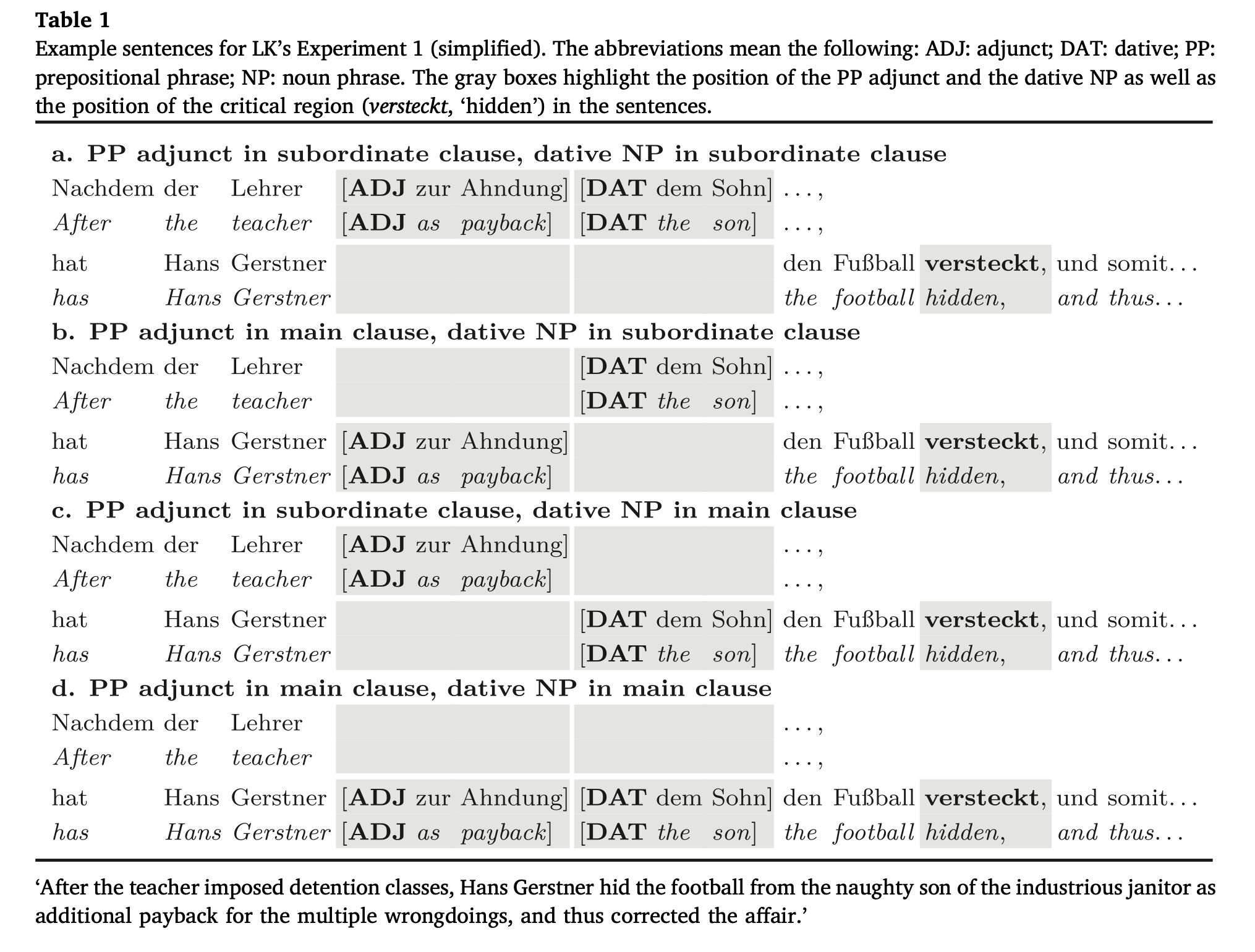
FIGURE 2.20: The experiment design in Experiment 1 of Levy and Keller (2013). The figure is re-used with permission from S. Vasishth et al. (2018) (License number 5211790221849).
Some pre-processing has to be carried out to do the t-tests needed to answer these questions. First, load the data, create a condition column, and then examine the resulting structure of the data frame:
data("df_levykeller13E1")
head(df_levykeller13E1)
## subj item dat adj TFT
## 1 1 1 main main 594
## 2 1 2 main sub 472
## 3 1 3 sub main 600
## 4 1 5 sub sub 768
## 5 1 6 main main 1190
## 6 1 7 main sub 318As will become clear below, it is convenient to recode the \(2\times 2\) design in terms of the four conditions labeled a-d.
## create a condition column:
df_levykeller13E1$cond <-
  factor(ifelse(df_levykeller13E1$dat == "sub" &
                  df_levykeller13E1$adj == "sub", "a",
    ifelse(df_levykeller13E1$dat == "sub" &
             df_levykeller13E1$adj == "main", "b",
      ifelse(df_levykeller13E1$dat == "main" &
               df_levykeller13E1$adj == "sub", "c",
        ifelse(df_levykeller13E1$dat == "main" &
                 df_levykeller13E1$adj == "main", "d", "NA")
      )
    )
  ))
## sanity check:
xtabs(~ cond + adj, df_levykeller13E1)
## adj
## cond main sub
## a 0 168
## b 168 0
## c 0 168
## d 168 0xtabs(~ cond + dat, df_levykeller13E1)## dat
## cond main sub
## a 0 168
## b 0 168
## c 168 0
## d 168 0Notice that each of the 28 subjects sees each condition six times. This is a Latin square design, which means that there should be \(6\times 4=24\) items. You must check this!
t(xtabs(~subj+cond,df_levykeller13E1))## subj
## cond 1 2 3 4 5 6 7 8 9 10 11 12 13 14 15 16 17 18 19
## a 6 6 6 6 6 6 6 6 6 6 6 6 6 6 6 6 6 6 6
## b 6 6 6 6 6 6 6 6 6 6 6 6 6 6 6 6 6 6 6
## c 6 6 6 6 6 6 6 6 6 6 6 6 6 6 6 6 6 6 6
## d 6 6 6 6 6 6 6 6 6 6 6 6 6 6 6 6 6 6 6
## subj
## cond 20 21 22 23 24 25 26 27 28
## a 6 6 6 6 6 6 6 6 6
## b 6 6 6 6 6 6 6 6 6
## c 6 6 6 6 6 6 6 6 6
## d 6 6 6 6 6 6 6 6 6The repeated measurements from each subject in each condition is problematic for the t-test: the t-test assumes that each subject delivers exactly one data point per condition. Mathematically, what’s assumed in the t-test is that for \(i=1,\dots,28\) subjects, we have four vectors of length 28, one for each condition:
- \(x_{a,1},\dots,x_{a,28}\)
- \(x_{b,1},\dots,x_{b,28}\)
- \(x_{c,1},\dots,x_{c,28}\)
- \(x_{d,1},\dots,x_{d,28}\)
Instead, what we have is four vectors, each of length \(28\times 6\). For example, look at condition a’s data:
length(subset(df_levykeller13E1,cond=="a")$TFT)## [1] 16828*6## [1] 168What is necessary here is to modify the data so as to get one single value for each participant in each condition. To achieve this format, the data must be aggregated: restructure the data so that each subject’s response for each of the four conditions is the mean of the six repetitions. An analysis using data aggregated by participant is often called a by-participant (or by-subject) analysis:
bysubj <- aggregate(TFT ~ subj + cond,
  mean,
  data = df_levykeller13E1
)
head(bysubj)
## subj cond TFT
## 1 1 a 601.7
## 2 2 a 798.3
## 3 3 a 640.7
## 4 4 a 732.7
## 5 5 a 1255.7
## 6 6 a 385.3Now, each subject delivers exactly one data point per condition, as the t-test demands.
length(subset(bysubj,cond=="a")$TFT)## [1] 28Notice that now we have no column any more indicating which items the subjects saw—this information has disappeared because for each subject, we took the average over all the six items for each condition. We have lost information; as will be discussed in later chapters, this loss of information can have far-reaching, adverse consequences for statistical inference.
t(xtabs(~subj+cond,bysubj))## subj
## cond 1 2 3 4 5 6 7 8 9 10 11 12 13 14 15 16 17 18 19
## a 1 1 1 1 1 1 1 1 1 1 1 1 1 1 1 1 1 1 1
## b 1 1 1 1 1 1 1 1 1 1 1 1 1 1 1 1 1 1 1
## c 1 1 1 1 1 1 1 1 1 1 1 1 1 1 1 1 1 1 1
## d 1 1 1 1 1 1 1 1 1 1 1 1 1 1 1 1 1 1 1
## subj
## cond 20 21 22 23 24 25 26 27 28
## a 1 1 1 1 1 1 1 1 1
## b 1 1 1 1 1 1 1 1 1
## c 1 1 1 1 1 1 1 1 1
## d 1 1 1 1 1 1 1 1 1The main effects and interactions can be visualized as in Figure 2.21.

FIGURE 2.21: Visualizing the aggregated data from the four conditions in the Levy and Keller (2013) Experiment 1 design allows us to graphically summarize the statistical comparisons of interest: the main effects of the two factors, and their interactions.
The main effect of dative is asking whether the average of the two dat:main conditions (the dative nouns appearing in the main clause) is different from the average of the two dat:sub conditions (dative appearing in the subordinate clause). In terms of the means of the four conditions labeled a-d, the null hypothesis is then:
\[\begin{equation} H_{0,MEdat}: \frac{\mu_a + \mu_b}{2} = \frac{\mu_c + \mu_d}{2} \end{equation}\]
The paired t-test can be used to test this main effect. It will be convenient to obtain the reading times for each condition, and just do paired t-tests. (Each of the main effects and the interaction are going to be paired t-tests.)
cond_a<-subset(bysubj,cond=="a")$TFT
cond_b<-subset(bysubj,cond=="b")$TFT
cond_c<-subset(bysubj,cond=="c")$TFT
cond_d<-subset(bysubj,cond=="d")$TFT
Here is the computation for the main effect of the dative noun:
## main effect of dative:
mean_ab<-(cond_a+cond_b)/2
mean_cd<-(cond_c+cond_d)/2

MEdat_res<-t.test(mean_ab,mean_cd,paired=TRUE)
summary_ttest(MEdat_res)
## [1] "t(27)=3.14 p=0.004"
## [1] "est.: 107.98 [37.36,178.61] ms"Levy and Keller (2013) report (their Table 6) a main effect of dative as having an estimate of \(102.48\) ms (no confidence interval is reported), with a p-value below \(0.01\). The small difference between their estimate and ours is because they analyzed unaggregated data with a linear mixed model. Their analysis is actually the better way to analyze these data, as we will discuss later in this book.
The main effect of adjunct is asking whether the average of the two adj:main conditions is different from the average of the two adj:sub conditions.
\[\begin{equation} H_{0,MEadj}: \frac{\mu_a + \mu_c}{2} = \frac{\mu_b + \mu_d}{2} \end{equation}\]
This main effect can be tested as follows:
mean_ac<-(cond_a+cond_c)/2
mean_bd<-(cond_b+cond_d)/2
MEadj_res<-t.test(mean_bd,mean_ac,paired=TRUE)
summary_ttest(MEadj_res)
## [1] "t(27)=-0.7 p=0.487"
## [1] "est.: -18.38 [-71.88,35.13] ms"Levy and Keller (2013) also report a non-significant effect estimate of 16.28 ms, so this approximately matches our estimate.
Finally, the interaction of the two factors (call it \(dat\times adj\)) is asking whether the adjunct effect within dat:main has the same value as the adjunct effect in dat:sub. In other words, the interaction is testing for no difference between two differences:
\[\begin{equation} H_{0,dat\times adj}: (\mu_a - \mu_b) = (\mu_c - \mu_d) \end{equation}\]
Another way to write this null hypothesis is as testing whether the difference between the two differences is 0:
\[\begin{equation} H_{0,dat\times adj}: (\mu_a - \mu_b) - (\mu_c - \mu_d) = 0 \end{equation}\]
The implementation of the t-test works like this:
diff_ab<-cond_a-cond_b
diff_cd<-cond_c-cond_d
INTdatxadj_res<-t.test(diff_ab,diff_cd,paired=TRUE)
summary_ttest(INTdatxadj_res)
## [1] "t(27)=-1.27 p=0.216"
## [1] "est.: -88.61 [-232,54.78] ms"Levy and Keller (2013) report a non-significant estimate of \(-96.82\) ms for the interaction. This also approximately matches our calculations.
To summarize, the three tests showed the following estimates:
- main effect of dative: 107.98 [37.36,178.61] ms. t(27)=3.14
- main effect of adjunct: -18.38 [-71.88,35.13] ms. t(27)= -0.7
- interaction: -88.61 [-232,54.78] ms. t(27)= -1.27
The above estimates and t-values suggest that we do have estimates that are consistent with a main effect of dat. Regarding the main effect of adj, there is no evidence against the null hypothesis of no difference. The interaction t-test also shows no evidence against the null hypothesis of no difference. So the data are only partly consistent with the authors’ predictions.
As an aside, notice that a repeated measures ANOVA could alternatively be used (instead of the three paired t-tests). An interesting point to notice here is that the F-scores that the repeated measures ANOVA returns below are the squares of the t-values we found above. This is because the paired t-tests we carried out above are identical to the ANOVA.
library(rstatix)##
## Attache Paket: 'rstatix'## Das folgende Objekt ist maskiert 'package:MASS':
##
## select## Das folgende Objekt ist maskiert 'package:stats':
##
## filterbysubj2 <- aggregate(TFT ~ subj + adj + dat,
mean,
data = df_levykeller13E1
)
subj_anova<-anova_test(data = bysubj2,
dv = TFT,
wid = subj,
within = c(adj,dat)
)
get_anova_table(subj_anova)## ANOVA Table (type III tests)
##
## Effect DFn DFd F p p<.05 ges
## 1 adj 1 27 0.497 0.487 0.000828
## 2 dat 1 27 9.842 0.004 * 0.028000
## 3 adj:dat 1 27 1.608 0.216 0.005000The broader lesson here is that one can break down a design with a factorial design to a series of paired t-tests. Although it is extremely easy to analyze factorial designs like these with paired t-tests, there is an important price to be paid. The price is inflation of Type I error probability.
2.7.2 A complication with multiple t-tests: Inflation of Type I error probability
Each of the three hypothesis tests has a Type I error probability set at \(0.05\). Once the three hypothesis tests are carried out, the probability space is as shown in Figure 2.22. The way to interpret the probability space is as follows: Each time that a hypothesis is tested, if the null hypothesis is in fact true, we can reject it incorrectly with probability 0.05, and accept it correctly with probability 0.95. Each successive hypothesis test takes us further down the tree, and the binary branches represent all the possible paths that could be taken. Thus, if we want to compute the probability of correctly failing to reject the null in all three hypothesis tests assuming that the null is true, we simply multiply the three probabilities 0.95 to get 0.8574. Subtracting one from this quantity gives us the probability of rejecting at least one null hypothesis incorrectly.
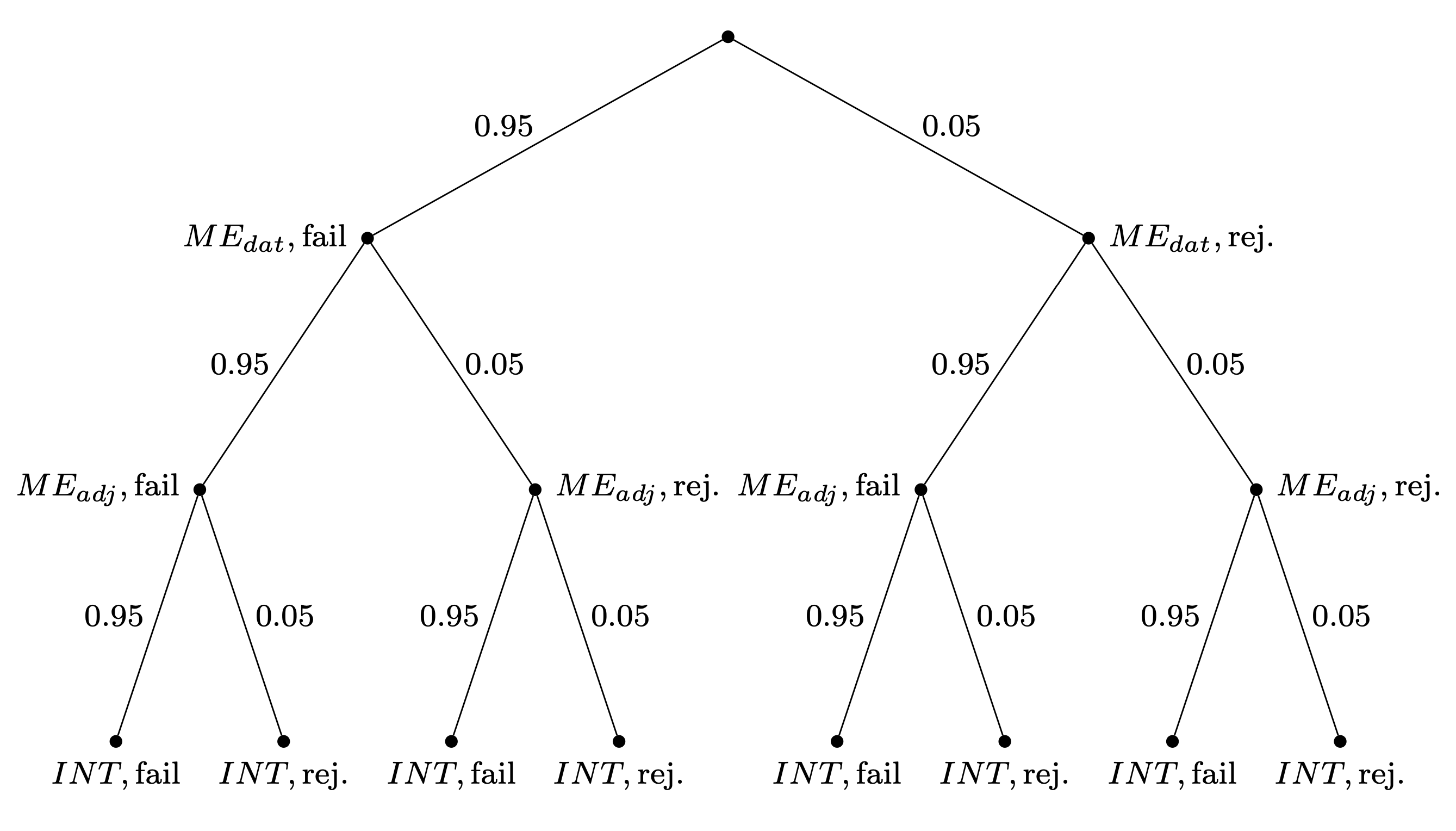
FIGURE 2.22: The probability space representing three successive independent hypothesis tests when all null hypotheses are true, and Type I error probability is 0.05. Each hypothesis can either be rejected (rej.) or fail to be rejected (fail).
The probability of rejecting at least one of the three hypotheses incorrectly is no longer \(0.05\), but rather:
\[\begin{equation} 1-0.95^3 = 0.1426 \end{equation}\]
This inflated Type I error probability can become very serious; for example, Levy and Keller (2013) carried out 32 hypothesis tests; this results in an inflated Type I error probability of
\[\begin{equation} 1-0.95^{32} = 0.8063 \end{equation}\]
That is an 80% probability of incorrectly rejecting at least one of the hypotheses tested! It is not unheard of to run 120 hypothesis tests in a single paper (e.g., B. Dillon et al. 2012). That would be a Type I error probability of 0.998 of rejecting at least one null hypothesis incorrectly. One is essentially sure to claim a significant effect incorrectly.
A standard approach to adjusting to this inflation is to use the Bonferroni correction: divide the standard Type I error by the number of tests, and use this corrected probability as the new Type I error. For example, in Levy and Keller (2013), the corrected \(\alpha\) for 32 hypothesis tests would be 0.05/32=0.0016. In B. Dillon et al. (2012), the corrected \(\alpha\) value would be 0.05/120=0.0004; under the corrected \(\alpha\), only one of the \(120\) tests comes out significant. When carrying out multiple statistical tests, a corrected \(\alpha\) to interpret multiple comparisons.
2.7.3 Analyzing a \(2\times 2\times 2\) repeated measures design using paired t-tests
Even more complex designs can be analyzed using paired t-tests. For example, Fedorenko, Gibson, and Rohde (2006) report a self-paced reading study with eight conditions. There are free factors:
- Memory load: One noun in memory set or three nouns:
- easy: Joel
- hard: Joel-Greg-Andy
- Noun type: either proper name or occupation:
- name: Joel-Greg-Andy
- occ: poet-cartoonist-voter
- Relative clause type:
- subject relative
- object relative
The relative clause sentences are the following; the reading time is measured in the relative clause regions who consulted the cardiologist and who the cardiologist consulted.
Subject-extracted: The physician | who consulted the cardiologist | checked the files | in the office.
Object-extracted: The physician | who the cardiologist consulted | checked the files | in the office.
The authors had two versions of each of the two relative clause types, but we ignore that detail here. Another problem in the data is that subject 1 delivers twice as much data as the other subjects; this could be due to two subjects being misclassified as subject 1. But we ignore this problem in the data as well.
First, load and examine the data:
data("df_fedorenko06")
head(df_fedorenko06)
## rctype nountype load item subj region RT
## 2 obj name hard 16 1 2 4454
## 6 subj name hard 4 1 2 5718
## 10 subj name easy 10 1 2 2137
## 14 subj name hard 20 1 2 903
## 18 subj name hard 12 1 2 1837
## 22 subj occ hard 19 1 2 1128As explained above, we have a \(2\times 2\times 2\) design: rctype [obj,subj] \(\times\) nountype [name, occupation] \(\times\) load [hard,easy]. Region 2 is the critical region, the entire relative clause, and RT is the reading time for this region. Subject and item columns are self-explanatory.
The paired t-test can be used repeatedly to compute the main effects and interactions. This will be assigned as an exercise at the end of this chapter. Here, we want to focus on one interesting analysis in the original paper. The result from that paper is summarized in the quote below (emphasis ours):
“The most interesting result presented here is an interaction between syntactic complexity and the memory- noun/sentence-noun similarity during the critical region of the linguistic materials in the hard-load (three memory-nouns) conditions: people processed object-extracted relative clauses more slowly when they had to maintain a set of nouns that were similar to the nouns in the sentence than when they had to maintain a set of nouns that were dissimilar from the nouns in the sentence; in contrast, for the less complex subject-extracted relative clauses, there was no reading time difference between the similar and dissimilar memory load conditions. In the easy-load (one memory-noun) conditions, no interaction between syntactic complexity and memory-noun/sentence-noun similarity was observed. These results provide evidence against the hypothesis whereby there is a pool of domain-specific verbal working memory resources for sentence comprehension, contra Caplan and Waters (1999). ”
If the analyses described in the quote above are to be carried out using t-tests (or repeated measures ANOVA), the approach that must be taken is to subset the data such that there are two \(2\times 2\) subsetted data sets: one for the hard memory conditions and the other for the easy memory conditions. Then, one can investigate the interaction between the relative clause type (syntactic complexity) and the noun type (proper name vs. occupation) by computing aggregated differences between (i) the relative clause type in Noun Type occupation, and (i) the relative clause type in Noun Type proper name.
fed06hard<-subset(df_fedorenko06,load=="hard")

## Compute difference between
## object relative (obj) and subject relative (subj)
## in Noun Type occupation:
RCocc<-aggregate(RT~subj+rctype,
                 mean,data=subset(fed06hard,
                                  nountype=="occ"))
diff_occ_hard<-subset(RCocc,rctype=="obj")$RT-
  subset(RCocc,rctype=="subj")$RT

## Compute difference between OR and SR
## in Noun Type proper name:
RCname<-aggregate(RT~subj+rctype,
                  mean,data=subset(fed06hard,
                                   nountype=="name"))
diff_name_hard<-subset(RCname,rctype=="obj")$RT-
  subset(RCname,rctype=="subj")$RT

## by-subject interaction:
hardINTres<-t.test(diff_name_hard,
                   diff_occ_hard,paired=TRUE)
summary_ttest(hardINTres)
## [1] "t(43)=-2.13 p=0.039"
## [1] "est.: -404.81 [-787.91,-21.71] ms"One can also investigate the interaction between RC type and Noun Type in the easy conditions:
fed06easy <- subset(df_fedorenko06,
                    load == "easy")

## Compute difference between OR and SR
## in Noun Type occupation:
RCocc <- aggregate(RT ~ subj + rctype,
                   mean, data = subset(fed06easy,
                                       nountype == "occ"))
diff_occ_easy <- subset(RCocc, rctype == "obj")$RT -
  subset(RCocc, rctype == "subj")$RT

## Compute difference between OR and SR
## in Noun Type proper name:
RCname <- aggregate(RT ~ subj + rctype,
                    mean, data = subset(fed06easy,
                                        nountype == "name"))
diff_name_easy <- subset(RCname,
                         rctype == "obj")$RT -
  subset(RCname, rctype == "subj")$RT

## by-subject interaction:
easyINTres <- t.test(diff_name_easy,
                     diff_occ_easy,
                     paired = TRUE)
summary_ttest(easyINTres)
## [1] "t(43)=-0.1 p=0.922"
## [1] "est.: -15.16 [-326.05,295.74] ms"Based on these aggregated by-subjects analyses, it would be tempting to conclude, as Fedorenko, Gibson, and Rohde (2006) did, that there is a significant interaction in the hard conditions but not in the easy conditions. However, there are at least two problems here. First, the paired t-test (or the identical test, the repeated measures ANOVA) has a serious limitation: it is ignoring the by-item variability (because that is averaged out); later we will see that once one takes all sources of variance into account simultaneously, the picture changes dramatically. Second, the authors implicitly assume that the difference between a significant effect in the hard conditions and the non-significant effect in the easy conditions is itself significant—we will see below that this conclusion is not warranted in the present case.
In summary, the (paired) t-test is a quick and easy tool for comparing means from two conditions, and even relatively complex designs can be analyzed. In fact, a well-known mathematical psychologist once told the first author of this book: “If you need to run anything more complex than a t-test, you are asking the wrong question.” Indeed, many scientists have had long and successful careers with just the t-test as their entire statistical tool. However, as they say, if all you have is a hammer, everything starts to look like a nail. As we show in this book, much important information is lost when one attempts to boil the data down to fit the constraints of the t-test.
A further point is that the t-test is often used incorrectly. Some of the most common mistakes are discussed next.