Chapter 19 Mixture models

Mixture models integrate multiple data generating processes into a single model. This is especially useful in cases where the data alone don’t allow us to fully identify which observations belong to which process. Mixture models are important in cognitive science because many theories of cognition assume that the behavior of subjects in certain tasks is determined by an interplay of different cognitive processes (e.g., response times in schizophrenia in Levy et al. 1993; retrieval from memory in sentence processing in McElree 2000; Nicenboim and Vasishth 2018; fast choices in Ollman 1966; Dutilh et al. 2011). It is important to stress that a mixture distribution of observations is an assumption of the latent process developing trial by trial based on a given theory—it doesn’t necessarily represent the true generative process. The role of Bayesian modeling is to help us understand the extent to which this assumption is well-founded, by using posterior predictive checks and comparing different models.

We focus here on the case where we have only two components; each component represents a distinct cognitive process based on the domain knowledge of the researcher. The vector $\mathbf{z}$ serves as an indicator variable that indicates which of the mixture components an observation $y_n$ belongs to ($n=1,\dots,N$ is the number of data points). We assume two components, and thus each $z_n$ can be either $0$ or $1$ (this will allows us to generate $z_n$ with a Bernoulli distribution). We also assume two different generative processes, $p_1$ and $p_2$, which generate different distributions of the observations based on a vector of parameters indicated by $\Theta_{1}$ and $\Theta_{2}$, respectively. These two processes occur with probability $\theta$ and $1-\theta$, and each observation is generated as follows:

\[\begin{equation} \begin{aligned} z_n \sim \mathit{Bernoulli}(\theta)\\ y_n \sim \begin{cases} p_1(\Theta_1), & \text{ if } z_n =1 \\ p_2(\Theta_2), & \text{ if } z_n=0 \end{cases} \end{aligned} \tag{19.1} \end{equation}\]

We focus on only two components because this type of model is already hard to fit and as we show in this chapter, it requires plenty of prior information to being able to sample from the posterior in most applied situations. However, the approach presented here can in principle be extended to a larger number of mixtures by replacing the Bernoulli distribution by a categorical one. This can be done if the number of components in the mixture is finite and also determined by the researcher.

In order to fit this model, we need to estimate the posterior of each of the parameters contained in the vectors $\Theta_{1}$ and $\Theta_{2}$ (intercepts, slopes, group-level effects, etc.), the probability $\theta$, and the indicator variable that corresponds to each observation $z_n$. One issue that presents itself here is that $z_n$ must be a discrete parameter, and Stan only allows continuous parameters. This is because Stan’s algorithm requires the derivatives of the (log) posterior distribution with respect to all parameters, and discrete parameters are not differentiable (since they have “breaks”). In probabilistic programming languages like WinBUGS and JAGS (Lunn et al. 2012; Plummer 2016), discrete parameters are possible to use; but not in Stan. In Stan, we can circumvent this issue by marginalizing out the indicator variable $z$.⁵⁸ If $p_1$ appears in the mixture with probability $\theta$, and $p_2$ with probability $1-\theta$, then the joint likelihood is defined as a function of $\Theta$ (which concatenates the mixing probability, $\theta$, and the parameters of the $p_{1}$ and $p_{2}$, $\Theta_1$ and $\Theta_2$), and importantly $z_n$ “disappears”:

\[\begin{equation} p(y_n | \Theta) = \theta \cdot p_1(y_n| \Theta_1) + (1-\theta) \cdot p_2(y_n | \Theta_2) \end{equation}\]

The intuition behind this formula is that each likelihood function, $p_1$, $p_2$ is weighted by its probability of being the relevant generative process. For our purposes, it suffices to say that marginalization works; the reader interested in the mathematics behind marginalization is directed to the further reading section at the end of the chapter.⁵⁹

Even though Stan cannot fit a model with the discrete indicator of the latent class $\mathbf{z}$ that we used in equation (19.1), this equation will prove very useful when we want to generate synthetic data.

In the following sections, we model a well-known phenomenon (i.e., the speed-accuracy trade-off) assuming an underlying finite mixture process. We start from the verbal description of the model, and then implement the model in Stan step by step.

19.1 A mixture model of the speed-accuracy trade-off: The fast-guess model account

When we are faced with multiple choices that require an immediate decision, we can speed up the decision at the expense of accuracy and become more accurate at the expense of speed; this is called the speed-accuracy trade-off (Wickelgren 1977). The most popular class of models that can incorporate both response times and accuracy, and give an account for the speed-accuracy trade-off is the class of sequential sampling models, which include the drift diffusion model (Ratcliff 1978), the linear ballistic accumulator (Brown and Heathcote 2008), and the log-normal race model (Heathcote and Love 2012; Rouder et al. 2015), which we discuss in chapter 20; for a review see Ratcliff et al. (2016).

However, an alternative model that has been proposed in the past is Ollman’s simple fast-guess model (Ollman 1966; Yellott 1967, 1971).⁶⁰ Although it has mostly fallen out of favor (but see Dutilh et al. 2011 for a more modern variant of this model), it presents a very simple framework using finite mixture modeling that can also account for the speed-accuracy trade-off. In the next sections, we’ll use this model to exemplify the use of finite mixtures to represent different cognitive processes.

19.1.1 The global motion detection task

One way to examine the behavior of human and primate subjects when faced with two-alternative forced choices is the detection of the global motion of a random dot kinematogram (Britten et al. 1993). In this task, a subject sees a number of random dots on the screen. A proportion of dots move in a single direction (e.g., right) and the rest move in random directions. The subject’s goal is to estimate the overall direction of the movement. One of the reasons for the popularity of this task is that it permits the fine-tuning of the difficulty of trials (Dutilh et al. 2019): The task is harder when the proportion of dots that move coherently (the level of coherence) is lower; see Figure 19.1.

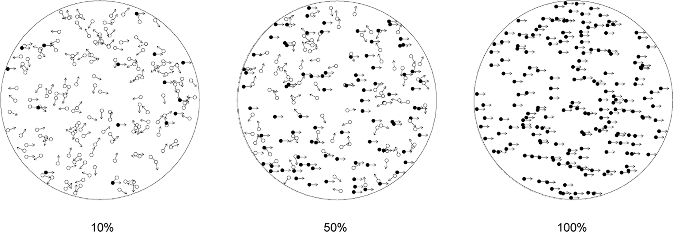
Three levels of difficulty of the global motion detection task. The figures show a consistent movement to the right with three levels of coherence (10%, 50%, and 100%). The subjects see the dots moving in the direction indicated by the arrows. The subjects do not see the arrows and all the dots look identical in the actual task. Adapted from Han et al. (2018); licensed under CC BY 4.0 (https://creativecommons.org/licenses/by/4.0/).

FIGURE 19.1: Three levels of difficulty of the global motion detection task. The figures show a consistent movement to the right with three levels of coherence (10%, 50%, and 100%). The subjects see the dots moving in the direction indicated by the arrows. The subjects do not see the arrows and all the dots look identical in the actual task. Adapted from Han et al. (2018); licensed under CC BY 4.0 (https://creativecommons.org/licenses/by/4.0/).

Ollman’s (1966) fast-guess model assumes that the behavior in this task (and in any other choice task) is governed by two distinct cognitive processes: (i) a guessing mode, and (ii) a task-engaged mode. In the guessing mode, responses are fast and accuracy is at chance level. In the task-engaged mode, responses are slower and accuracy approaches 100%. This means that intermediate values of response times and accuracy can only be achieved by mixing responses from the two modes. Further assumptions of this model are that response times depend on the difficulty of the choice, and that the probability of being on one of the two states depend on the speed incentives during the instructions.

To simplify matters, we ignore the possibility that the accuracy of the choice is also affected by the difficulty of the choice. Also, we ignore the possibility that subjects might be biased to one specific response in the guessing mode, but see exercise 19.3.

19.1.1.1 The data set

We implement the assumptions behind Ollman’s fast-guess model and examine its fit to data of a global motion detection task from Dutilh et al. (2019).

The data set from Dutilh et al. (2019) contains approximately 2800 trials of each of the 20 subjects participating in a global motion detection task and can be found in df_dots in the bcogsci package. There were two level of coherence, yielding hard and easy trials (diff), and the trials where done under instructions that emphasized either accuracy or speed (emphasis). More information about the data set can be found by accessing the documentation for the data set (by typing ?df_dots in the R console, assuming that the bcogsci package is installed).

data("df_dots") 
df_dots

## # A tibble: 56,097 × 12
##    subj diff  emphasis    rt   acc fix_dur stim  resp  trial block
##   <int> <chr> <chr>    <dbl> <int>   <dbl> <chr> <chr> <int> <int>
## 1     1 easy  speed      482     1   0.738 R     R         1     6
## 2     1 hard  speed      602     1   0.784 R     R         2     6
## 3     1 hard  speed      381     1   0.651 R     R         3     6
##   block_trial bias 
##         <int> <chr>
## 1           1 no   
## 2           2 no   
## 3           3 no   
## # ℹ 56,094 more rows

We might think that if the fast-guess model were true, we would see a bimodal distribution, when we plot a histogram of the data. Unfortunately, when two similar distributions are mixed, we won’t necessarily see any apparent bimodality; see Figure 19.2.


ggplot(df_dots, aes(rt)) +
  geom_histogram()

FIGURE 19.2: Distribution of response times in the data of the global motion detection task in Dutilh et al. (2019).

However, Figure 19.3 reveals that incorrect responses were generally faster, and this was especially true when the instructions emphasized accuracy.


ggplot(df_dots, aes(x = factor(acc), y = rt)) +
  geom_point(position = position_jitter(width = .4, height = 0),
             alpha = .5) +
  facet_wrap(diff ~ emphasis) +
  xlab("Accuracy") +
  ylab("Response time")

FIGURE 19.3: The distribution of response times by accuracy in the data of the global motion detection task in Dutilh et al. (2019).

19.1.2 A very simple implementation of the fast-guess model

The description of the model makes it clear that an ideal subject who never guesses has a response time that depends only on the difficulty of the trial. As we did in previous chapters, we assume that response times are log-normally distributed, and for simplicity we start by modeling the behavior of a single subject:

\[\begin{equation} rt_n \sim \mathit{LogNormal}(\alpha + \beta \cdot x_n, \sigma) \end{equation}\]

In the previous equation, $x$ is larger for difficult trials. If we center $x$, $\alpha$ represents the average logarithmic transformed response time for a subject engaged in the task, and $\beta$ is the effect of trial difficulty on log-response time. We assume a non-deterministic process, with a noise parameter $\sigma$. See also Box 4.3 for more information about log-normally distributed response times.

Alternatively, a subject that guesses in every trial would show a response time distribution that is independent of the difficulty of the trial:

\[\begin{equation} rt_n \sim \mathit{LogNormal}(\gamma, \sigma_2) \end{equation}\]

Here $\gamma$ represents the the average logarithmic transformed response time when a subject only guesses. We assume that responses from the guessing mode might have a different noise component than from the task-engaged mode.

The fast-guess model makes the assumption that during a task, a single subject would behave in these two ways: They would be engaged in the task a proportion of the trials and would guess on the rest of the trials. This means that for a single subject, there is an underlying probability of being engaged in the task, $p_{task}$, that determines whether they are actually choosing ($z=1$) or guessing ($z=0$):

\[\begin{equation} z_n \sim \mathit{Bernoulli}(p_{task}) \end{equation}\]

The value of the parameter $z$ in every trial determines the behavior of the subject. This means that the distribution that we observe is a mixture of the two distributions presented before:

\[\begin{equation} rt_n \sim \begin{cases} \mathit{LogNormal}(\alpha + \beta \cdot x_n, \sigma), & \text{ if } z_n =1 \\ \mathit{LogNormal}(\gamma, \sigma_2), & \text{ if } z_n=0 \end{cases} \tag{19.2} \end{equation}\]

In order to have a Bayesian implementation, we also need to define some priors. We use priors that encode what we know about reaction time experiments. These priors are slightly more informative than the ones that we used in section 4.2, but they still can be considered regularizing priors. One can verify this by performing prior predictive checks. As we increase the complexity of our models, it’s worth spending some time designing more realistic priors. These will speed up computation and in some cases they will be crucial for solving convergence problems.

\[\begin{equation} \begin{aligned} \alpha &\sim \mathit{Normal}(6, 1)\\ \beta &\sim \mathit{Normal}(0, .1)\\ \sigma &\sim \mathit{Normal}_+(.5, .2) \end{aligned} \end{equation}\]

\[\begin{equation} \begin{aligned} \gamma &\sim \mathit{Normal}(6, 1)\\ \sigma_2 &\sim \mathit{Normal}_+(.5, .2) \end{aligned} \end{equation}\]

For now, we allow all values for the probability of having an engaged response having equal likelihood; we achieve this by setting the following prior to $p_{task}$:

\[\begin{equation} p_{task} \sim \mathit{Beta}(1, 1) \end{equation}\]

This represents a flat, uninformative prior over the probability parameter $p_{task}$.

Before we fit our model to the real data, we generate synthetic data to make sure that our model is working as expected.

We first define the number of observations, predictors, and fixed point values for each of the parameters. We assume $1000$ observations and two levels of difficulty, coded $-0.5$ (easy) and $0.5$ (hard). The point values chosen for the parameters are relatively realistic (based on our previous experience on reaction time experiments). Although in the priors we try to encode the range of possible values for the parameters, in this simulation we assume only one instance of this possible range:

N <- 1000
# level of difficulty:
x <- c(rep(-.5, N/2), rep(.5, N/2)) 
# Parameters true values:
alpha <- 5.8
beta <- 0.05
sigma <- .4
sigma2 <- .5
gamma <- 5.2
p_task <- .8
# Median time
c("engaged" = exp(alpha), "guessing" = exp(gamma))

##  engaged guessing 
##      330      181

For generate a mixture of response times, we use the indicator of a latent class, z.

z <- rbern(n = N, prob = p_task)
rt <- if_else(z == 1,
             rlnorm(N,
                    meanlog = alpha + beta * x,
                    sdlog = sigma),
             rlnorm(N, 
                    meanlog = gamma,
                    sdlog = sigma2))
df_dots_simdata1 <- tibble(trial = 1:N, x = x, rt = rt)

We verify that our simulated data is realistic, that is, it’s in the same range as the original data; see Figure 19.4.

ggplot(df_dots_simdata1, aes(rt)) +
  geom_histogram()

FIGURE 19.4: Response times in the simulated data (df_dots_simdata1) that follows the fast-guess model.

To implement the mixture model defined in equation (3.10) in Stan, the discrete parameter $z$ needs to be marginalized out:

\[\begin{equation} \begin{aligned} p(rt_n | \Theta) &= p_{task} \cdot LogNormal(rt_n | \alpha + \beta \cdot x_n, \sigma) +\\ & (1 - p_{task}) \cdot LogNormal(rt_n | \gamma, \sigma_2) \end{aligned} \end{equation}\]

In addition, Stan requires the likelihood to be defined in log-space:

\[\begin{equation} \begin{aligned} \log(p(rt | \Theta)) &= \log(p_{task} \cdot LogNormal(rt_n | \alpha + \beta \cdot x_n, \sigma) +\\ & (1 - p_{task}) \cdot LogNormal(rt_n | \gamma, \sigma_2)) \end{aligned} \end{equation}\]

A “naive” implementation in Stan would look like the following (recall that _lpdf functions provide log-transformed densities):

target += log(
        p_task * exp(lognormal_lpdf(rt[n] | alpha + x[n] * beta, sigma)) +
              (1-p_task) * exp(lognormal_lpdf(rt[n] | gamma, sigma2)));

However, we need to take into account that $log(A \pm B)$ can be numerically unstable (i.e., prone to underflow/ overflow, see Blanchard, Higham, and Higham 2020). Stan provides several functions to deal with different special cases of logarithms of sums and differences. Here we need log_sum_exp(x, y) that corresponds to log(exp(x) + exp(y)) and log1m(x) that corresponds to log(1-x).

First, we need to take into account that the first summand of the logarithm, p_task * exp(lognormal_lpdf(rt[n] | alpha + x[n] * beta, sigma)) corresponds to exp(x), and the second one, (1-p_task) * exp(lognormal_lpdf(rt[n] | gamma, sigma2)) to exp(y) in log_sum_exp(x, y). This means that we need to first apply the logarithm to each of them to use them as arguments of log_sum_exp(x, y):

target += log_sum_exp(
              log(p_task) + lognormal_lpdf(rt[n] | alpha + 
              x[n] * beta, sigma),
              log(1-p_task) + lognormal_lpdf(rt[n] | gamma, sigma2));

Now we can just replace log(1-p_task) by the more stable log1m(p_task):

target += log_sum_exp(
               log(p_task) + lognormal_lpdf(rt[n] | alpha + 
               x[n] * beta, sigma),
               log1m(p_task) + lognormal_lpdf(rt[n] | gamma, sigma2));

The complete model (mixture_rt.stan) is shown below:

data {
  int<lower = 1> N;
  vector[N] x;
  vector[N] rt;
}
parameters {
  real alpha;
  real beta;
  real<lower = 0> sigma;
  real gamma; //guessing
  real<lower = 0> sigma2;
  real<lower = 0, upper = 1> p_task;
}
model {
  // priors for the task component
  target += normal_lpdf(alpha | 6, 1);
  target += normal_lpdf(beta | 0, .1);
  target += normal_lpdf(sigma | .5, .2)
    - normal_lccdf(0 | .5, .2);
  // priors for the guessing component
  target += normal_lpdf(gamma | 6, 1);
  target += normal_lpdf(sigma2 | .5, .2)
    - normal_lccdf(0 | .5, .2);
  target += beta_lpdf(p_task | 1, 1);
  // likelihood
  for(n in 1:N)
    target +=
      log_sum_exp(log(p_task) +
                  lognormal_lpdf(rt[n] | alpha + x[n] * beta, sigma),
                  log1m(p_task) +
                  lognormal_lpdf(rt[n] | gamma, sigma2));
}

Call the Stan model mixture_rt.stan, and fit it to the simulated data. First, we set up the simulated data as a list structure:

ls_dots_simdata <- list(N = N, rt = rt, x = x)

Then fit the model:

mixture_rt <- system.file("stan_models",
                        "mixture_rt.stan",
                        package = "bcogsci")
fit_mix_rt <- stan(mixture_rt, data = ls_dots_simdata)

## Warning: The largest R-hat is 1.74, indicating chains have not mixed.
## Running the chains for more iterations may help. See
## https://mc-stan.org/misc/warnings.html#r-hat
## 
##  Warning: Bulk Effective Samples Size (ESS) is too low, indicating
## posterior means and medians may be unreliable. Running the chains for
## more iterations may help. See
## https://mc-stan.org/misc/warnings.html#bulk-ess
## 
##  Warning: Tail Effective Samples Size (ESS) is too low, indicating
## posterior variances and tail quantiles may be unreliable. Running the
## chains for more iterations may help. See
## https://mc-stan.org/misc/warnings.html#tail-ess

There are a lot of warnings, the Rhats are too large, and number of effective samples is too low:

print(fit_mix_rt)

##            mean     2.5%    97.5% n_eff Rhat
## alpha      5.67     5.01     6.01     3 2.20
## beta       0.04    -0.11     0.18     5 1.33
## sigma      0.39     0.19     0.56     2 2.26
## gamma      5.72     5.34     5.99     2 2.38
## sigma2     0.43     0.23     0.55     3 2.21
## p_task     0.40     0.12     0.81    14 1.12
## lp__   -6386.07 -6390.83 -6382.91    11 1.13

The traceplots show clearly that the chains aren’t mixing; see Figure 19.5.

traceplot(fit_mix_rt) +
  scale_x_continuous(breaks = NULL)

FIGURE 19.5: Traceplots from the model mixture_rt.stan fit to simulated data.

The problem with this model is that the mixture components (i.e., the fast-guesses and the engaged mode) are underlyingly exchangeable (see Box 5.1) and thus the posterior is multi-modal and the model does not converge. Each chain doesn’t know how each component was identified by the rest of the chains. However, we do have information that can identify the components: According to the theoretical model, we know that the average response in the engaged mode, represented by $\alpha$, should be slower than the average response in the guessing mode, $\gamma$.

Even though the theoretical model assumes that guesses are faster than engaged responses, this is not explicit in our computational model. That is, our model lacks some of the theoretical information that we have, namely that the distribution of engaged response times should be slower than the distribution of guesses times. This can be encoded with a strong prior for $\gamma$, where we assume that its prior distribution is truncated on an upper bound by the value of $\alpha$:

\[\begin{equation} \gamma \sim \mathit{Normal}(6, 1), \text{for } \gamma < \alpha \end{equation}\]

This would be enough to make the model to converge.

Another softer constraint that we could add to our implementation is the assumption that subjects are generally more likely to be trying to do the task than just guessing. If this assumption is correct, we also improve the accuracy of our estimation of the posterior of the model. (The opposite is also true: If subjects are not trying to do the task, this assumption will be unwarranted and our prior information will lead us further from the “true” values of the parameters). The following prior has the probability density concentrated near $1$.

\[\begin{equation} p_{task} \sim \mathit{Beta}(8, 2) \end{equation}\]

Plotting this prior confirms where most of the probability mass lies; see Figure 19.6.


plot(function(x) dbeta(x, 8, 2), ylab = "density" , xlab= "probability")
`## Warning: Line is too long.`

$A density plot for the $Beta(8,2)$ prior on $p_{task}$.$

FIGURE 19.6: A density plot for the $Beta(8,2)$ prior on $p_{task}$.

The Stan code for this model is shown below as mixture_rt2.stan.

data {
  int<lower = 1> N;
  vector[N] x;
  vector[N] rt;
}
parameters {
  real alpha;
  real beta;
  real<lower = 0> sigma;
  real<upper = alpha> gamma;
  real<lower = 0> sigma2;
  real<lower = 0, upper = 1> p_task;
}
model {
  target += normal_lpdf(alpha | 6, 1);
  target += normal_lpdf(beta | 0, .3);
  target += normal_lpdf(sigma | .5, .2)
    - normal_lccdf(0 | .5, .2);
  target += normal_lpdf(gamma | 6, 1) -
    normal_lcdf(alpha | 6, 1);
  target += normal_lpdf(sigma2 | .5, .2)
    - normal_lccdf(0 | .5, .2);
  target += beta_lpdf(p_task | 8, 2);
  for(n in 1:N)
    target +=
      log_sum_exp(log(p_task) +
                  lognormal_lpdf(rt[n] | alpha + x[n] * beta, sigma),
                  log1m(p_task) +
                  lognormal_lpdf(rt[n] | gamma, sigma2)) ;
}

Once we change the upper bound of gamma in the parameters block, we also need to truncate the distribution in the model block by correcting the PDF with its CDF. This correction is carried out using the CDF because we are truncating the distribution at the right-hand side; recall that earlier we used the complement of the CDF when we truncate a distribution at the left-hand side); see Box 4.1.

  target += normal_lpdf(gamma | 6, 1) -
    normal_lcdf(alpha | 6, 1);

Fit this model (call it mixture_rt2.stan) to the same simulated data set that we used before:

mixture_rt2 <- system.file("stan_models",
                        "mixture_rt2.stan",
                        package = "bcogsci")
fit_mix_rt2 <- stan(mixture_rt2, data = ls_dots_simdata)

Now the summaries and traceplots look fine; see Figure 19.7.

print(fit_mix_rt2)

##            mean     2.5%    97.5% n_eff Rhat
## alpha      5.84     5.75     5.95  1263    1
## beta       0.05    -0.02     0.14  1265    1
## sigma      0.39     0.30     0.44   832    1
## gamma      5.26     4.90     5.57   989    1
## sigma2     0.47     0.35     0.58  1221    1
## p_task     0.70     0.36     0.91   872    1
## lp__   -6387.28 -6391.94 -6384.55  1209    1

traceplot(fit_mix_rt2) + 
  scale_x_continuous(breaks = NULL)

FIGURE 19.7: Traceplots from the model mixture_rt2.stan fit to simulated data.

19.1.3 A multivariate implementation of the fast-guess model

A problem with the previous implementation of the fast-guess model is that we ignore the accuracy information in the data. We can implement a version that is closer to the verbal description of the model: In particular, we also want to model the fact that accuracy is at chance level in the fast-guessing mode and that accuracy approaches 100% during the task-engaged mode.

This means that the mixture affects two pairs of distributions:

\[\begin{equation} z_n \sim \mathit{Bernoulli}(p_{task}) \end{equation}\]

The response time distribution

and an accuracy distribution

\[\begin{equation} acc_n \sim \begin{cases} \mathit{Bernoulli}(p_{correct}), & \text{ if } z_n =1 \\ \mathit{Bernoulli}(0.5), & \text{ if } z_n=0 \end{cases} \tag{19.4} \end{equation}\]

We have a new parameter $p_{correct}$, which represent the probability of making a correct answer in the engaged mode. The verbal description says that it is closer to 100%, and here we have the freedom to choose whatever prior we believe represents for us values that are close to 100% accuracy. We translate this belief into a prior as follows; our prior choice is relatively informative but does not impose a hard constraint; if a subject consistently shows relatively low (or high) accuracy, $p_{correct}$ will change accordingly:

\[\begin{equation} p_{correct} \sim \mathit{Beta}(995, 5) \end{equation}\]

In our simulated data, we assume that the global motion detection task is done by a very accurate subject, with an accuracy of 99.9%.

First, simulate reaction times, as done earlier:

N <- 1000
x <- c(rep(-.5, N/2), rep(.5, N/2)) # difficulty
alpha <- 5.8
beta <- 0.05
sigma <- 0.4
sigma2 <- 0.5
gamma <- 5.2 # fast guess location
p_task <- 0.8 # prob of being on task
z <- rbern(n = N, prob = p_task)
rt <- if_else(z == 1,
             rlnorm(N,
                    meanlog = alpha + beta * x,
                    sdlog = sigma),
             rlnorm(N, 
                    meanlog = gamma,
                    sdlog = sigma2))

Simulate accuracy and include both reaction times and accuracy in the simulated data set:

p_correct <- 0.999
acc <- ifelse(z, rbern(n = N, p_correct),
                  rbern(n = N, 0.5))
df_dots_simdata3 <- tibble(trial = 1:N,
                           x = x,
                           rt = rt,
                           acc = acc) %>%
                    mutate(diff = if_else(x == 0.5, "hard", "easy"))

Plot the simulated data in Figure 19.8. This time we can see the effect of task difficulty on the simulated response times and accuracy:

ggplot(df_dots_simdata3, aes(x = factor(acc), y = rt)) +
  geom_point(position = position_jitter(width = .4, height = 0),
             alpha = .5) +
  facet_wrap(diff ~ .) +
  xlab("Accuracy") +
  ylab("Response time")

FIGURE 19.8: Response times by accuracy accounting for task difficulty in the simulated data (df_dots_simdata3) that follows the fast-guess model.

Next, we need to marginalize out the discrete parameters from both pairs of distributions.

\[\begin{equation} \begin{aligned} p(rt, acc | \Theta) = & p_{task} \cdot \\ & LogNormal(rt_n | \alpha + \beta \cdot x_n, \sigma) \cdot \\ & Bernoulli(acc_n | p_{correct}) \\ & +\\ & (1 - p_{task}) \cdot \\ & LogNormal(rt_n | \gamma, \sigma_2) \cdot\\ & Bernoulli(acc_n | .5) \end{aligned} \end{equation}\]

In log-space:

\[\begin{equation} \begin{aligned} \log(p(rt, acc | \Theta)) = \log(\exp(&\\ & \log(p_{task}) +\\ &\log(LogNormal(rt_n | \alpha + \beta * x_n, \sigma)) + \\ &\log(Bernoulli(acc_n | p_{correct})))\\ +&\\ \exp(&\\ & \log(1 - p_{task}) + \\ & \log(LogNormal(rt_n |\gamma, \sigma_2)) + \\ & \log(Bernoulli(acc_n | .5)))\\ )& \\ \end{aligned} \end{equation}\]

Our model translates to the following Stan code (mixture_rtacc.stan):

data {
  int<lower = 1> N;
  vector[N] x;
  vector[N] rt;
  array[N] int acc;
}
parameters {
  real alpha;
  real beta;
  real<lower = 0> sigma;
  real<upper = alpha> gamma;
  real<lower = 0> sigma2;
  real<lower = 0, upper = 1> p_correct;
  real<lower = 0, upper = 1> p_task;
}
model {
  target += normal_lpdf(alpha | 6, 1);
  target += normal_lpdf(beta | 0, .3);
  target += normal_lpdf(sigma | .5, .2)
    - normal_lccdf(0 | .5, .2);
  target += normal_lpdf(gamma | 6, 1) -
    normal_lcdf(alpha | 6, 1);
  target += normal_lpdf(sigma2 | .5, .2)
    - normal_lccdf(0 | .5, .2);
  target += beta_lpdf(p_correct | 995, 5);
  target += beta_lpdf(p_task | 8, 2);
  for(n in 1:N)
    target +=
      log_sum_exp(log(p_task) +
                 lognormal_lpdf(rt[n] | alpha + x[n] * beta, sigma) +
                 bernoulli_lpmf(acc[n] | p_correct),
                 log1m(p_task) +
                 lognormal_lpdf(rt[n] | gamma, sigma2) +
                 bernoulli_lpmf(acc[n] | .5));
}

Next, set up the data in list format:

ls_dots_simdata <- list(N = N,
                        rt = rt,
                        x = x,
                        acc = acc)

Then fit the model:

mixture_rtacc <- system.file("stan_models",
                        "mixture_rtacc.stan",
                        package = "bcogsci")
fit_mix_rtacc <- stan(mixture_rtacc, data = ls_dots_simdata)

We see that our model can be fit to both response times and accuracy, and its parameters estimates have sensible values (given the fixed parameters we used to generate our simulated data).

print(fit_mix_rtacc)

##               mean     2.5%    97.5% n_eff Rhat
## alpha         5.78     5.75     5.81  4244    1
## beta          0.06     0.00     0.12  5103    1
## sigma         0.39     0.37     0.42  5140    1
## gamma         5.19     5.08     5.30  3699    1
## sigma2        0.51     0.45     0.58  4455    1
## p_correct     0.99     0.99     1.00  4662    1
## p_task        0.81     0.77     0.85  5422    1
## lp__      -6609.94 -6614.50 -6607.19  1835    1

We will evaluate the recovery of the parameters more carefully when we deal with the hierarchical version of the fast-guess model in section 19.1.5. Before we extend this model hierarchically, let us also take into account the instructions given to the subjects.

19.1.4 An implementation of the fast-guess model that takes instructions into account

The actual global motion detection experiment that we started with has another manipulation that can help us to evaluate better the fast-guess model. In some trials, the instructions emphasized accuracy (e.g., “Be as accurate as possible.”) and in others speed (e.g., “Be as fast as possible.”). The fast-guess model also assumes that the probability of being in one of the two states depends on the speed incentives given during the instructions. This entails that now $p_{task}$ depends on the instructions $x_2$, where we encode a speed incentive with $-0.5$ and an accuracy incentive with $0.5$. Essentially, we need to fit the following regression:

\[\begin{equation} \alpha_{task} + x_2 \cdot \beta_{task} \end{equation}\]

As we did with MPT models in the previous chapter (in section 18.2.3), we need to bound the previous regression between 0 and 1; we achieve this using the logistic or inverse logit function:

\[\begin{equation} p_{task} = logit^{-1}(\alpha_{task} + x_2 \cdot \beta_{task}) \end{equation}\]

This means that we need to interpret $\alpha_{task} + x_2 \cdot \beta_{task}$ in log-odds space, which has the range $(-\infty, \infty)$ rather than the probability space $[0,1]$; also see section 18.2.3.

The likelihood (defined before in section 19.1.3) now depends on the value of $x_{2}$ for the specific row:

\[\begin{equation} z_n \sim \mathit{Bernoulli}(p_{{task}_n}) \end{equation}\]

A response time distribution is defined:

and an accuracy distribution is defined as well:

\[\begin{equation} acc_n \sim \begin{cases} \mathit{Bernoulli}(p_{correct}), & \text{ if } z_n =1 \\ \mathit{Bernoulli}(0.5), & \text{ if } z_n=0 \end{cases} \end{equation}\]

The only further change in our model is that rather than a prior on $p_{task}$, we now need priors for $\alpha_{task}$ and $\beta_{task}$, which are on the log-odds scale.

For $\beta_{task}$, we assume an effect that can be rather large and we won’t assume a direction a priori (for now):

\[\begin{equation} \beta_{task} \sim \mathit{Normal}(0, 1) \end{equation}\]

This means that the subject could be affected by the instructions in the expected way, with an increased probability to be task-engaged, leading to better accuracy when the instructions emphasize accuracy ($\beta_{task} >0$). Alternatively, the subject might be behaving in an unexpected way, with a decreased probability to be task-engaged, leading to worse accuracy when the instructions emphasize accuracy ($\beta_{task} <0$). The latter situation, $\beta_{task} <0$, could represent the instructions being misunderstood. It’s certainly possible to include priors that encode the expected direction of the effect instead: $\mathit{Normal}_{+}(0,1)$. Unless there is a compelling reason to constrain the prior in this way, following Cromwell’s rule (Box 6.2), we leave open the possibility of the $\beta$ parameter having negative values.

How can we choose a prior for $\alpha_{task}$ that encodes the same information that we had in the previous model in $p_{task}$? One possibility is to create an auxiliary parameter $p_{btask}$, that represents the baseline probability of being engaged in the task, with the same prior that we use in the previous section, and then transform it to an unconstrained space for our regression with the logit function:

\[\begin{equation} \begin{aligned} &p_{btask} \sim \mathit{\mathit{Beta}}(8, 2)\\ &\alpha_{task} = logit(p_{btask}) \end{aligned} \end{equation}\]

To verify that our priors make sense, in Figure 19.9 we plot the difference in prior predicted probability of being engaged in the task under the two emphasis conditions:

Ns <- 1000 # number of samples for the plot
# Priors
p_btask <- rbeta(n = Ns, shape1 = 8, shape2 = 2)
beta_task <- rnorm(n = Ns, mean = 0, sd = 1)
# Predicted probability of being engaged
p_task_easy <- plogis(qlogis(p_btask) + 0.5 * beta_task)
p_task_hard <- plogis(qlogis(p_btask) + -0.5 * beta_task)
# Predicted difference
diff_p_pred <- tibble(diff = p_task_easy - p_task_hard)

diff_p_pred %>%
  ggplot(aes(diff)) +
  geom_histogram()

The difference in prior predicted probability of being engaged in the task under the two emphasis conditions for the simulated data (diff_p_pred) that follows the fast-guess model.

FIGURE 19.9: The difference in prior predicted probability of being engaged in the task under the two emphasis conditions for the simulated data (diff_p_pred) that follows the fast-guess model.

Figure 19.9 shows that we are predicting a priori that the difference in $p_{task}$ will tend to be smaller than $\pm 0.3$, which seems to make sense intuitively. If we had more information about the likely range of variation, we could of course have adapted the prior to reflect that belief.

We are ready to generate a new data set, by deciding on some fixed values for $\beta_{task}$ and $p_{btask}$:

N <- 1000
x <- c(rep(-0.5, N/2), rep(0.5, N/2)) # difficulty
x2 <- rep(c(-0.5, 0.5), N/2) # instructions
# Verify that the predictors are crossed:
predictors <- tibble(x, x2)
xtabs(~ x + x2, predictors)

##       x2
## x      -0.5 0.5
##   -0.5  250 250
##   0.5   250 250

alpha <- 5.8
beta <- 0.05
sigma <- 0.4
sigma2 <- 0.5
gamma <- 5.2 
p_correct <- 0.999
# New true values:
p_btask <- 0.85
beta_task <- 0.5
# Generate data:
alpha_task <- qlogis(p_btask)
p_task <- plogis(alpha_task + x2 * beta_task)
z <- rbern(N, prob = p_task)
rt <- ifelse(z,
             rlnorm(N, meanlog = alpha + beta * x, sdlog = sigma),
             rlnorm(N, meanlog = gamma, sdlog = sigma2))
acc <- ifelse(z, rbern(N, p_correct),
                 rbern(N, 0.5))
df_dots_simdata4 <- tibble(trial = 1:N,
                           x = x,
                           rt = rt,
                           acc = acc,
                           x2 = x2) %>%
          mutate(diff = if_else(x == 0.5, "hard", "easy"),
                 emphasis = ifelse(x2 == 0.5, "accuracy", "speed"))

We can generate a plot now where both the difficulty of the task and the instructions are manipulated; see Figure 19.10.

ggplot(df_dots_simdata4, aes(x = factor(acc), y = rt)) +
  geom_point(position = position_jitter(width = .4, height = 0),
             alpha = .5) +
  facet_wrap(diff ~ emphasis) +
  xlab("Accuracy") +
  ylab("Response time")

Response times and accuracy by the difficulty of the task and the instructions type for the simulated data (df_dots_simdata4) that follows the fast-guess model.

FIGURE 19.10: Response times and accuracy by the difficulty of the task and the instructions type for the simulated data (df_dots_simdata4) that follows the fast-guess model.

In the Stan implementation, log_inv_logit(x) is applying the logistic (or inverse logit) function to x to transform it into a probability and then applying the logarithm; log1m_inv_logit(x) is applying the logistic function to x, and then applying the logarithm to its complement $(1 - p)$. We do this because rather than having p_task in probability space, we have lodds_task in log-odds space:

real lodds_task = logit(p_btask) + x2[n] * beta_task;

The parameter lodds_task estimates the mixing probabilities in log-odds:

target += log_sum_exp(log_inv_logit(lodds_task) + ..., 
          log1m_inv_logit(lodds_task) + ...)

We also add a generated quantities block that can be used for further (prior or posterior) predictive checks. In this block we do use z as an indicator of the latent class (task-engaged mode or fast-guessing mode), since we do not estimate z, but rather generate it based on the parameter’s posteriors.

We use the dummy variable onlyprior to indicate whether we use the data or we only sample from the priors. One can always do the predictive checks in R, transforming the code that we wrote for the simulation into a function, and writing the priors in R. However, it can be simpler to take advantage of Stan output format and rewrite the code in Stan. One downside of this is that the stanfit object that stores the model output can become too large for the memory of the computer.

data {
  int<lower = 1> N;
  vector[N] x;
  vector[N] rt;
  array[N] int acc;
  vector[N] x2; //speed or accuracy emphasis
  int<lower = 0, upper = 1> onlyprior;
}
parameters {
  real alpha;
  real beta;
  real<lower = 0> sigma;
  real<upper = alpha> gamma;
  real<lower = 0> sigma2;
  real<lower = 0, upper = 1> p_correct;
  real<lower = 0, upper = 1> p_btask;
  real beta_task;
}
model {
  target += normal_lpdf(alpha | 6, 1);
  target += normal_lpdf(beta | 0, .1);
  target += normal_lpdf(sigma | .5, .2)
    - normal_lccdf(0 | .5, .2);
  target += normal_lpdf(gamma | 6, 1)-
  normal_lcdf(alpha | 6, 1);
  target += normal_lpdf(sigma2 | .5, .2)
    - normal_lccdf(0 | .5, .2);
  target += normal_lpdf(beta_task | 0, 1);
  target += beta_lpdf(p_correct | 995, 5);
  target += beta_lpdf(p_btask | 8, 2);
  if(onlyprior != 1)
    for(n in 1:N){
      real lodds_task = logit(p_btask) + x2[n] * beta_task;
      target +=
        log_sum_exp(log_inv_logit(lodds_task)+
                 lognormal_lpdf(rt[n] | alpha + x[n] * beta, sigma) +
                 bernoulli_lpmf(acc[n] | p_correct),
                 log1m_inv_logit(lodds_task) +
                 lognormal_lpdf(rt[n] | gamma, sigma2) +
                 bernoulli_lpmf(acc[n] | .5));
    }
}
generated quantities {
  array[N] real rt_pred;
  array[N] real acc_pred;
  array[N] int z;
  for(n in 1:N){
    real lodds_task = logit(p_btask) + x2[n] * beta_task;
    z[n] = bernoulli_rng(inv_logit(lodds_task));
    if(z[n]==1){
      rt_pred[n] = lognormal_rng(alpha + x[n] * beta, sigma);
      acc_pred[n] = bernoulli_rng(p_correct);
    } else{
      rt_pred[n] = lognormal_rng(gamma, sigma2);
      acc_pred[n] = bernoulli_rng(.5);
    }
  }
}

We save the code as mixture_rtacc2.stan, and before fitting it to the simulated data, we perform prior predictive checks.

19.1.4.1 Prior predictive checks

Generate prior predictive distributions, by setting onlyprior to 1.

ls_dots_simdata <- list(N = N,
                        rt = rt,
                        x = x,
                        x2 = x2,
                        acc = acc,
                        onlyprior = 1) 
mixture_rtacc2 <- system.file("stan_models", 
                        "mixture_rtacc2.stan", 
                        package = "bcogsci")

fit_mix_rtacc2_priors <- stan(mixture_rtacc2,
                         data = ls_dots_simdata,
                         chains = 4, iter = 2000)

We plot prior predictive distributions of response times as follows in Figure 19.11, by setting y = rt using ppd_dens_overlay().

rt_pred <- extract(fit_mix_rtacc2_priors)$rt_pred
ppd_dens_overlay(rt_pred[1:100,]) +
  coord_cartesian(xlim = c(0, 2000))

FIGURE 19.11: Prior predictive distributions of response times (using mixture_rtacc2.stan) that follows the fast-guess model.

Some of the predictive data sets contain responses that are too large, and some of them have too much probability mass close to zero, but there is nothing clearly wrong in the prior predictive distributions (considering that the model hasn’t “seen” the data yet).

If we want to plot the prior predicted distribution of differences in response time conditioning on task difficulty, we need to define a new function. Then we use the bayesplot function ppc_stat() that takes as an argument of stat any summary function; see Figure 19.12.

meanrt_diff <- function(rt){
  mean(rt[x == .5]) -
    mean(rt[x == -.5])
} 
ppd_stat(rt_pred, stat = meanrt_diff)

FIGURE 19.12: Prior predicted distribution (using mixture_rtacc2.stan) of differences in response time, conditioning on task difficulty.

We find that the range of response times look reasonable. There are, however, always more checks that can be done; examples are plotting other summary statistics, or predictions conditioned on other aspects of the data.

19.1.4.2 Fit to simulated data

Fit the model to data, by setting onlyprior = 0:

ls_dots_simdata <- list(N = N,
                        rt = rt,
                        x = x,
                        x2 = x2,
                        acc = acc,
                        onlyprior = 0)

fit_mix_rtacc2 <- stan(mixture_rtacc2, data = ls_dots_simdata)

print(fit_mix_rtacc2,
      pars = c("alpha", "beta", "sigma", "gamma", "sigma2",
               "p_correct", "p_btask", "beta_task"))

##           mean 2.5% 97.5% n_eff Rhat
## alpha     5.82 5.78  5.85  5098    1
## beta      0.05 0.00  0.11  5977    1
## sigma     0.40 0.38  0.42  4591    1
## gamma     5.12 5.00  5.24  3205    1
## sigma2    0.46 0.38  0.53  3661    1
## p_correct 0.99 0.99  1.00  3721    1
## p_btask   0.86 0.83  0.89  3977    1
## beta_task 0.62 0.16  1.10  4921    1

We see that we fit the model without problems. Before we evaluate the recovery of the parameters more carefully, we implement a hierarchical version of the fast-guess model.

19.1.5 A hierarchical implementation of the fast-guess model

So far we have evaluated the behavior of one simulated subject. We discussed before (in the context of distributional regression models, in section 5.2.6, and in the MPT modeling chapter 18) that, in principle, every parameter in a model can be made hierarchical. However, this doesn’t guarantee that we’ll learn anything from the data for those parameters, or that our model will converge. A safe approach here is to start simple, using simulated data. Despite the fact that convergence with simulated data does not guarantee the convergence of the same model with real data, in our experience the reverse is in general true.

For our hierarchical version, we assume that both response times and the effect of task difficulty vary by subject, and that different subjects have different guessing times. This entails the following change to the response time distribution:

\[\begin{equation} rt_n \sim \begin{cases} \mathit{LogNormal}(\alpha + u_{subj[n],1} + x_n \cdot (\beta + u_{subj[n], 2}), \sigma), & \text{ if } z_n =1 \\ \mathit{LogNormal}(\gamma + u_{subj[n], 3}, \sigma_2), & \text{ if } z_n=0 \end{cases} \end{equation}\]

We assume that the three vectors of $u$ (adjustment to the intercept and slope of the task-engaged distribution, and the adjustment to the guessing time distribution) follow a multivariate normal distribution centered on zero. For simplicity and lack of any prior knowledge about this experiment design and method, we assume the same (weakly informative) prior distribution for the three variance components and the same regularizing LKJ prior for the three correlations between the adjustments ($\rho_{u_{1,2}}, \rho_{u_{1,3}}, \rho_{u_{2,3}}$):

\[\begin{equation} \begin{aligned} \boldsymbol{u} &\sim\mathcal{N}(0, \Sigma_u)\\ \tau_{u_{1..3}} & \sim \mathit{ \mathit{Normal}}_+(0, 0.5)\\ \rho_u &\sim \mathit{LKJcorr}(2) \end{aligned} \end{equation}\]

Before we fit the model to the real data set, we simulate data again; this time we simulate 100 trials of each of 20 subjects.

# Build the fake stimuli
N_subj <- 20
N_trials <- 100
# Parameters true values
alpha <- 5.8
beta <- 0.05
sigma <- 0.4
sigma2 <- 0.5
gamma <- 5.2
beta_task <- 0.1
p_btask <- 0.85
alpha_task <- qlogis(p_btask)
p_correct <- 0.999
tau_u <- c(0.2, 0.005, 0.3)
rho <- 0.3

## Build the data set here:
N <- N_subj * N_trials
stimuli <- tibble(x = rep(c(rep(-.5, N_trials / 2),
                            rep(.5, N_trials / 2)), N_subj),
                  x2 = rep(rep(c(-.5, .5), N_trials / 2), N_subj),
                  subj = rep(1:N_subj, each = N_trials),
                  trial = rep(1:N_trials, N_subj)
                  )
stimuli

## # A tibble: 2,000 × 4
##       x    x2  subj trial
##   <dbl> <dbl> <int> <int>
## 1  -0.5  -0.5     1     1
## 2  -0.5   0.5     1     2
## 3  -0.5  -0.5     1     3
## # ℹ 1,997 more rows

# Build the correlation matrix for the adjustments u:
Cor_u <- matrix(rep(rho, 9), nrow = 3)
diag(Cor_u) <- 1
Cor_u

##      [,1] [,2] [,3]
## [1,]  1.0  0.3  0.3
## [2,]  0.3  1.0  0.3
## [3,]  0.3  0.3  1.0

# Variance covariance matrix for subjects:
Sigma_u <- diag(tau_u, 3, 3) %*% Cor_u %*% diag(tau_u, 3, 3)
# Create the correlated adjustments: 
u <- mvrnorm(n = N_subj, c(0, 0, 0), Sigma_u)
# Check whether they are correctly correlated
# (There will be some random variation,
# but if you increase the number of observations and
# the value of the correlation, you'll be able to obtain
# a more exact value below):
cor(u)

##       [,1]  [,2]  [,3]
## [1,] 1.000 0.514 0.314
## [2,] 0.514 1.000 0.245
## [3,] 0.314 0.245 1.000

# Check the SDs:
sd(u[, 1]); sd(u[, 2]); sd(u[, 3])

## [1] 0.221

## [1] 0.00586

## [1] 0.295

# Create the simulated data:
df_dots_simdata <- stimuli %>%
  mutate(z = rbern(N, prob = plogis(alpha_task + x2 * beta_task)),
         rt = ifelse(z,
             rlnorm(N, meanlog = alpha + u[subj, 1] +
                             (beta + u[subj, 2]) * x,
                    sdlog = sigma),
             rlnorm(N, meanlog = gamma + u[subj, 3],
                    sdlog = sigma2)),
         acc = ifelse(z, rbern(n = N, p_correct),
              rbern(n = N, 0.5)),
         diff = if_else(x == 0.5, "hard", "easy"),
         emphasis = ifelse(x2 == 0.5, "accuracy", "speed"))

Verify that the distribution of the simulated response times conditional on the simulated accuracy and the experimental manipulations make sense with the plot shown in Figure 19.13.

ggplot(df_dots_simdata, aes(x = factor(acc), y = rt)) +
  geom_point(position = position_jitter(width = .4, 
                                        height = 0), alpha = .5) +
  facet_wrap(diff ~ emphasis) +
  xlab("Accuracy") +
  ylab("Response time")

The distribution of response times conditional on the simulated accuracy and the experimental manipulations for the simulated hierarchical data (df_dots_simdata) that follows the fast-guess model.

FIGURE 19.13: The distribution of response times conditional on the simulated accuracy and the experimental manipulations for the simulated hierarchical data (df_dots_simdata) that follows the fast-guess model.

We implement the model in Stan as follows in mixture_h.stan. The hierarchical extension uses the Cholesky factorization for the group-level effects (as we did in section 11.1.3).

data {
  int<lower = 1> N;
  vector[N] x;
  vector[N] rt;
  array[N] int acc;
  vector[N] x2;
  int<lower = 1> N_subj;
  array[N] int<lower = 1, upper = N_subj> subj;
}
parameters {
  real alpha;
  real beta;
  real<lower = 0> sigma;
  real<upper = alpha> gamma;
  real<lower = 0> sigma2;
  real<lower = 0, upper = 1> p_correct;
  real<lower = 0, upper = 1> p_btask;
  real beta_task;
  vector<lower = 0>[3]  tau_u;
  matrix[3, N_subj] z_u;
  cholesky_factor_corr[3] L_u;
}
transformed parameters {
  matrix[N_subj, 3] u;
  u = (diag_pre_multiply(tau_u, L_u) * z_u)';
}
model {
  target += normal_lpdf(alpha | 6, 1);
  target += normal_lpdf(beta | 0, .1);
  target += normal_lpdf(sigma | .5, .2)
    - normal_lccdf(0 | .5, .2);
  target += normal_lpdf(gamma | 6, 1) -
    normal_lcdf(alpha | 6, 1);
  target += normal_lpdf(sigma2 | .5, .2)
    - normal_lccdf(0 | .5, .2);
  target += normal_lpdf(tau_u | 0, .5)
    - 3* normal_lccdf(0 | 0, .5);
  target += normal_lpdf(beta_task | 0, 1);
  target += beta_lpdf(p_correct | 995, 5);
  target += beta_lpdf(p_btask | 8, 2);
  target += lkj_corr_cholesky_lpdf(L_u | 2);
  target += std_normal_lpdf(to_vector(z_u));
  for(n in 1:N){
    real lodds_task = logit(p_btask) + x2[n] * beta_task;
    target +=
      log_sum_exp(log_inv_logit(lodds_task) +
          lognormal_lpdf(rt[n] | alpha + u[subj[n], 1] +
                         x[n] * (beta + u[subj[n], 2]), sigma) +
          bernoulli_lpmf(acc[n] | p_correct),
          log1m_inv_logit(lodds_task) +
          lognormal_lpdf(rt[n] | gamma + u[subj[n], 3], sigma2) +
          bernoulli_lpmf(acc[n] |.5));
  }
}
generated quantities {
  corr_matrix[3] rho_u = L_u * L_u';
}

Save the model code and fit it to the simulated data:

ls_dots_simdata <- list(N = N,
                        rt = df_dots_simdata$rt,
                        x = df_dots_simdata$x,
                        x2 = df_dots_simdata$x2,
                        acc = df_dots_simdata$acc,
                        subj = df_dots_simdata$subj,
                        N_subj = N_subj)
mixture_h <- system.file("stan_models",
                        "mixture_h.stan",
                        package = "bcogsci")
fit_mix_h <- stan(file = mixture_h,
                  data = ls_dots_simdata,
                  iter = 3000,
                  control = list(adapt_delta = .9))

Print the posterior summary:

print(fit_mix_h, pars = c("alpha", "beta", "sigma", "gamma",
                          "sigma2", "p_correct", "p_btask",
                          "beta_task", "tau_u",
                          "rho_u[1,2]", "rho_u[1,3]",
                          "rho_u[2,3]"))

##             mean  2.5% 97.5% n_eff Rhat
## alpha       5.78  5.68  5.88   910 1.00
## beta        0.06  0.02  0.10  7820 1.00
## sigma       0.39  0.37  0.41 12378 1.00
## gamma       5.21  5.05  5.37  3565 1.00
## sigma2      0.48  0.43  0.54  8221 1.00
## p_correct   1.00  0.99  1.00  9570 1.00
## p_btask     0.85  0.83  0.87  8538 1.00
## beta_task   0.11 -0.21  0.43 11280 1.00
## tau_u[1]    0.21  0.15  0.31  1591 1.00
## tau_u[2]    0.03  0.00  0.09  2711 1.00
## tau_u[3]    0.33  0.21  0.48  3127 1.00
## rho_u[1,2] -0.10 -0.76  0.63  8910 1.00
## rho_u[1,3]  0.22 -0.22  0.61  4427 1.00
## rho_u[2,3]  0.02 -0.73  0.74   672 1.01

We see that we can fit the hierarchical extension of our model to simulated data. Next we’ll evaluate whether we can recover the true values of the parameters.

19.1.5.1 Recovery of the parameters

By “recovering” the true values of the parameters, we mean that the true values are somewhere inside the bulk of the posterior distribution of the model.

We use mcmc_recover_hist to compare the posterior distributions of the relevant parameters of the model with their true values in Figure 19.14.

df_fit_mix_h <- fit_mix_h %>% as.data.frame() %>%
  select(c("alpha", "beta", "sigma", "gamma", "sigma2",
           "p_correct","p_btask", "beta_task", "tau_u[1]",
           "tau_u[2]", "tau_u[3]", "rho_u[1,2]", "rho_u[1,3]",
           "rho_u[2,3]"))
true_values <- c(alpha, beta, sigma, gamma, sigma2,
                p_correct, p_btask, beta_task, tau_u[1],
                tau_u[2], tau_u[3], rep(rho,3))
mcmc_recover_hist(df_fit_mix_h, true_values)

FIGURE 19.14: Posterior distributions of the main parameters of the mixture model fit_mix_h together with their true values.

The model seems to be underestimating the probability of subjects being correct (p_correct) and overestimating the probability of being engaged in the task (p_btask). However, the numerical differences are very small. We can be relatively certain that the model is not seriously misspecified. As mentioned in previous chapters, a more principled (and computationally demanding) approach uses simulation based calibration introduced in section 12.2 of chapter 12 (also see Talts et al. 2018; Schad, Betancourt, and Vasishth 2020).

19.1.5.2 Fitting the model to real data

After verifying that our model works as expected, we are ready to fit it to real data. We code the predictors $x$ and $x_2$ as we did for the simulated data:

df_dots <- df_dots %>%
  mutate(x = if_else(diff == "easy", -.5, .5),
         x2 = if_else(emphasis == "accuracy", .5, -.5))

The main obstacle now is that fitting the entire data set takes around 12 hours! We’ll sample 600 observations of each subject as follows:

df_dots_data_short <- df_dots %>%
  group_by(subj) %>% 
  sample_n(600)

ls_dots_data_short <-
  list(N = nrow(df_dots_data_short),
       rt = df_dots_data_short$rt,
       x = df_dots_data_short$x,
       x2 = df_dots_data_short$x2,
       acc = df_dots_data_short$acc,
       subj = as.numeric(df_dots_data_short$subj),
       N_subj = length(unique(df_dots_data_short$subj)))
fit_mix_data <- stan(file = mixture_h,
                     data = ls_dots_data_short,
                     chains = 4,
                     iter = 2000,
                     control = list(adapt_delta = .9,
                                    max_treedepth = 12))

## Warning: The largest R-hat is NA, indicating chains have not mixed.
## Running the chains for more iterations may help. See
## https://mc-stan.org/misc/warnings.html#r-hat
## 
##  Warning: Bulk Effective Samples Size (ESS) is too low, indicating
## posterior means and medians may be unreliable. Running the chains for
## more iterations may help. See
## https://mc-stan.org/misc/warnings.html#bulk-ess
## 
##  Warning: Tail Effective Samples Size (ESS) is too low, indicating
## posterior variances and tail quantiles may be unreliable. Running the
## chains for more iterations may help. See
## https://mc-stan.org/misc/warnings.html#tail-ess

The model has not converged at all!

print(fit_mix_data,
      pars = c("alpha", "beta", "sigma", "gamma", "sigma2",
               "p_correct","p_btask", "beta_task", "tau_u",
               "rho_u[1,2]", "rho_u[1,3]", "rho_u[2,3]"))

##            mean  2.5% 97.5% n_eff  Rhat
## alpha      6.36  6.19  6.48     3  2.15
## beta       0.10  0.03  0.15     2  3.07
## sigma      0.26  0.22  0.29     2 11.39
## gamma      6.18  6.05  6.34     2  2.28
## sigma2     0.28  0.19  0.42     2 19.27
## p_correct  0.93  0.87  1.00     2 16.66
## p_btask    0.85  0.68  0.94     2  8.25
## beta_task  1.83 -3.58  5.44     2 15.83
## tau_u[1]   0.14  0.09  0.21    21  1.08
## tau_u[2]   0.04  0.01  0.07     7  1.20
## tau_u[3]   0.26  0.11  0.70     2  3.11
## rho_u[1,2] 0.37 -0.17  0.77  2899  1.00
## rho_u[1,3] 0.19 -0.39  0.64    24  1.08
## rho_u[2,3] 0.17 -0.72  0.73     5  1.34

The traceplots in Figure 19.15 show that the chains are not mixing at all. It seems that the posterior is multimodal, and there are at least two combinations of parameters that would fit the data equally well.

traceplot(fit_mix_data) +
  scale_x_continuous(breaks = NULL)

Traceplots from the hierarchical model (mixture_h.stan) fit to (a subset) of the real data. The traceplot shows clearly that the posterior has at least two modes.

FIGURE 19.15: Traceplots from the hierarchical model (mixture_h.stan) fit to (a subset) of the real data. The traceplot shows clearly that the posterior has at least two modes.

What should we do now? It can be a good idea to back off and simplify the model. Once the simplified model converges, we can think about adding further complexity. The verbal description of our model says that the accuracy in the task-engaged mode should be close to 100%. To simplify the model, we’ll assume that it’s exactly 100%. This entails the following:

\[\begin{equation} p_{correct} = 1 \end{equation}\]

We adapt our Stan code in mixture_h2.stan, reflecting the assumption that p_correct has a fixed value; this parameter is now in a block called transformed data. There, we assign to p_correct the value of 1.

data {
  int<lower = 1> N;
  vector[N] x;
  vector[N] rt;
  array[N] int acc;
  vector[N] x2;
  int<lower = 1> N_subj;
  array[N] int<lower = 1, upper = N_subj> subj;
}
transformed data {
  real p_correct = 1;
}
parameters {
  real alpha;
  real beta;
  real<lower = 0> sigma;
  real<upper = alpha> gamma; //guessing
  real<lower = 0> sigma2;
  real<lower = 0, upper = 1> p_btask;
  real beta_task;
  vector<lower = 0>[3]  tau_u;
  matrix[3, N_subj] z_u;
  cholesky_factor_corr[3] L_u;
}
transformed parameters {
  matrix[N_subj, 3] u;
  u = (diag_pre_multiply(tau_u, L_u) * z_u)';
}
model {
  target += normal_lpdf(alpha | 6, 1);
  target += normal_lpdf(beta | 0, .1);
  target += normal_lpdf(sigma | .5, .2)
    - normal_lccdf(0 | .5, .2);
  target += normal_lpdf(gamma | 6, 1) -
    normal_lcdf(alpha | 6, 1);
  target += normal_lpdf(sigma2 | .5, .2)
    - normal_lccdf(0 | .5, .2);
  target += normal_lpdf(tau_u | 0, .5)
    - 3* normal_lccdf(0 | 0, .5);
  target += normal_lpdf(beta_task | 0, 1);
  target += beta_lpdf(p_btask | 8, 2);
  target += lkj_corr_cholesky_lpdf(L_u | 2);
  target += std_normal_lpdf(to_vector(z_u));
  for(n in 1:N){
    real lodds_task = logit(p_btask) + x2[n] * beta_task;
    target +=
      log_sum_exp(log_inv_logit(lodds_task) +
          lognormal_lpdf(rt[n] | alpha + u[subj[n], 1] +
                         x[n] * (beta + u[subj[n], 2]), sigma) +
          bernoulli_lpmf(acc[n] | p_correct),
          log1m_inv_logit(lodds_task) +
          lognormal_lpdf(rt[n] | gamma + u[subj[n], 3], sigma2) +
          bernoulli_lpmf(acc[n] |.5));
  }
}
generated quantities {
  corr_matrix[3] rho_u = L_u * L_u';
}

Fit the model again to the same data:

fit_mixs_data <- stan(file = mixture_h,
                     data = ls_dots_data_short,
                     chains = 4,
                     iter = 2000,
                     control = list(adapt_delta =.9,
                                    max_treedepth = 12))

The model has now converged:

print(fit_mixs_data,
      pars = c("alpha", "beta", "sigma", "gamma", "sigma2",
               "p_btask", "beta_task", "tau_u",
               "rho_u[1,2]", "rho_u[1,3]", "rho_u[2,3]"))

##            mean  2.5% 97.5% n_eff  Rhat
## alpha      6.36  6.29  6.46     3  1.62
## beta       0.09  0.05  0.15     2  3.06
## sigma      0.23  0.21  0.28     2 10.65
## gamma      6.24  6.06  6.35     2  2.70
## sigma2     0.36  0.19  0.42     2 19.35
## p_btask    0.74  0.68  0.91     2  8.71
## beta_task  1.84  0.67  5.32     2 11.78
## tau_u[1]   0.14  0.10  0.20    59  1.05
## tau_u[2]   0.03  0.01  0.06     5  1.27
## tau_u[3]   0.18  0.12  0.26     8  1.17
## rho_u[1,2] 0.39 -0.18  0.81  3652  1.00
## rho_u[1,3] 0.14 -0.28  0.54    17  1.09
## rho_u[2,3] 0.27 -0.31  0.75   519  1.03

The traceplots in Figure 19.16 show that this times the chains are mixing well.


traceplot(fit_mixs_data) +
  scale_x_continuous(breaks = NULL)

Traceplots from the simplified hierarchical model (mixture_h.stan, assuming that p_correct = 1) fit to (a subset) of the real data. The traceplot shows that chains are mixing well.

FIGURE 19.16: Traceplots from the simplified hierarchical model (mixture_h.stan, assuming that p_correct = 1) fit to (a subset) of the real data. The traceplot shows that chains are mixing well.

What can we say about the fit of the model now?

Under the assumptions that we have made (e.g., that there are two processing modes, response times are affected by the difficulty of the task in the task-engaged mode, accuracy is not affected by the difficulty of the task and is perfect at the task-engaged mode, etc.), we can look at the parameters and conclude the following:

The instructions seemed to have a strong effect on the processing mode of the subjects (beta_task is relatively high), and in the expected direction (emphasis in accuracy led to a higher probability to be in the task engaged mode).
The guessing mode seemed to be much noisier than the task-engaged mode (compare sigma with sigma2).
Slow subjects seemed to show a stronger effect of the experimental manipulation (rho_u1[1,2] is mostly positive).

If we want to know whether our model achieves descriptive adequacy, we need to look at the posterior predictive distributions of the model. However, by using posterior predictive checks, we won’t be able to conclude that our model is not overfitting. Our success in fitting the fast-guess model to real data does not entail that the model is a good account of the data. It just means that it’s flexible enough to fit the data. One further step could be to develop a competing model, and then comparing the performance of the models, using Bayes factors or cross validation.

19.1.5.3 Posterior predictive checks

For the posterior predictive checks, we can write the generated quantities block in a new file. The advantage is that we can generate as many observations as needed after estimating the parameters. There is no model block in the following Stan program and the parameters together with all the transformed parameters appear in the parameters block. We use the gqs() function in the rstan library, which allows us to use the posterior draws from a previously fitted model to generate posterior predicted data.

data {
  int<lower = 1> N;
  vector[N] x;
  vector[N] rt;
  array[N] int acc;
  vector[N] x2;
  int<lower = 1> N_subj;
  array[N] int<lower = 1, upper = N_subj> subj;
}
transformed data{
  real p_correct = 1;
}
parameters {
  real alpha;
  real beta;
  real<lower = 0> sigma;
  real<upper = alpha> gamma; //guessing
  real<lower = 0> sigma2;
  real<lower = 0, upper = 1> p_btask;
  real beta_task;
  vector<lower = 0>[3]  tau_u;
  matrix[3, N_subj] z_u;
  cholesky_factor_corr[3] L_u;
  matrix[N_subj, 3] u;
}
generated quantities {
  array[N] real rt_pred;
  array[N] real acc_pred;
  array[N] int z;
  for(n in 1:N){
    real lodds_task = logit(p_btask) + x2[n] * beta_task;
    z[n] = bernoulli_rng(inv_logit(lodds_task));
    if(z[n]==1){
      rt_pred[n] = lognormal_rng(alpha + u[subj[n],1] +
                               x[n] * (beta + u[subj[n], 2]), sigma);
      acc_pred[n] = bernoulli_rng(p_correct);
    } else{
      rt_pred[n] = lognormal_rng(gamma + u[subj[n], 3], sigma2);
      acc_pred[n] = bernoulli_rng(.5);
    }
  }
}

Generate responses from 500 simulated experiments as follows:

mixture_h2_gen <- system.file("stan_models",
                            "mixture_h2_gen.stan",
                            package = "bcogsci")
gen_model <- stan_model(mixture_h2_gen)
# The argument of the matrix `drop` needs to be set to FALSE,
# otherwise R will simplify the matrix into a vector.
# The two commas in the line below are not a mistake!
draws_par <- as.matrix(fit_mixs_data)[1:500, ,drop = FALSE]
gen_mix_data <- gqs(gen_model,
                    data = ls_dots_data_short,
                    draws = draws_par)

First, take a look at the general distribution of response times generated by the posterior predictive model and by our real data (Figure 19.17).

rt_pred <- extract(gen_mix_data)$rt_pred 
ppc_dens_overlay(y = ls_dots_data_short$rt, yrep = rt_pred[1:100,]) +
  coord_cartesian(xlim = c(0, 2000))

The posterior predictive distribution of the hierarchical fast-guess model (using mixture_h2_gen.stan) in comparison with the observed response times.

FIGURE 19.17: The posterior predictive distribution of the hierarchical fast-guess model (using mixture_h2_gen.stan) in comparison with the observed response times.

We see that the distribution of the observed response times is narrower than the predictive distribution. We are generating response times that are more spread out than the real data.

Next, examine the effect of the experimental manipulation in Figure 19.18: The posterior predictive check reveals that the model underestimates the observed effect of the experimental manipulation: the observed difference between response times is well outside the bulk of the predictive distribution.

meanrt_diff <- function(rt){
  mean(rt[ls_dots_data_short$x == .5]) -
    mean(rt[ls_dots_data_short$x == -.5])
}  
ppc_stat(ls_dots_data_short$rt,
         yrep = rt_pred,
         stat = meanrt_diff)

Posterior predictive distribution (using mixture_h2_gen.stan) of the difference in response time due to the experimental manipulation. The vertical bar shows the observed difference in the data.

FIGURE 19.18: Posterior predictive distribution (using mixture_h2_gen.stan) of the difference in response time due to the experimental manipulation. The vertical bar shows the observed difference in the data.

Another important posterior predictive check includes comparing the fit of the model using a quantile probability plot, which is presented in the next chapter.

We also look at some instances of the predictive distribution. Figure 19.19 shows a simulated data set in black overlaid onto the real observations in gray. As we noticed in Figure 19.17, the model is predicting less variability than what we find in the data, especially when the emphasis is on accuracy.

acc_pred <- extract(gen_mix_data)$acc_pred
df_dots_pred <-
  tibble(rt = ls_dots_data_short$rt,
         acc = ls_dots_data_short$acc,
         difficulty = ifelse(ls_dots_data_short$x == .5,
                             "hard", "easy"),
         emphasis = ifelse(ls_dots_data_short$x2 == -.5,
                           "speed", "accuracy"),
         acc_pred1 = acc_pred[1,],
         rt_pred1 = rt_pred[1,])

FIGURE 19.19: A simulated (posterior predictive) data set in black overlaid onto the observations in gray (based on mixture_h2_gen.stan).

If we would like to compare this model with a competing one using cross-validation, we would need to calculate the point-wise log-likelihood in the generated block:

generated quantities {
  array[N] real log_lik;
  for(n in 1:N){
    real lodds_task = logit(p_btask) + x2[n] * beta_task;
    log_lik[n] += log_sum_exp(log_inv_logit(lodds_task) +
                                lognormal_lpdf(rt[n] | alpha + u[subj[n], 1] +
                                                 x[n] * (beta + u[subj[n], 2]), sigma) +
                                bernoulli_lpmf(acc[n] | p_correct),
                              log1m_inv_logit(lodds_task) +
                                lognormal_lpdf(rt[n] | gamma + u[subj[n], 3], sigma2) +
                                bernoulli_lpmf(acc[n] |.5));
  }
}

It is important to bear in mind that we can only compare models on the same dependent variable(s). That is, we would need to compare this model with another one fit to the same dependent variables and also in the same scale: accuracy (0 or 1) and response time in milliseconds. This means that, for example, we cannot compare our fast-guess model with an accuracy-only model, for example. It also means that to compare our fast-guess model with a model based on left/right choices (known as stimulus coding, see section 20.1.1) and response times, we would need to reparameterize one of the two models; see exercise 20.3 in chapter 20.

To conclude, the fast-guess model shows a relatively decent fit to the data and is able to account for the speed-accuracy trade-off. The model shows some inaccuracies that could lead to its revision and improvement. To what extent the inaccuracies are acceptable or not depends on (i) the empirical finding that we want to account for (for example, we can already assume that the model will struggle to fit data sets that show slow errors); and (ii) its comparison with a competing account.

19.2 Summary

In this chapter, we learned to fit increasingly complex two-component mixture models using Stan, starting with a simple model and ending with a fully hierarchical model. We saw how to evaluate model fit using the usual prior and posterior predictive checks, and to investigate parameter recovery. Such mixture models are notoriously difficult to fit, but they have a lot of potential in cognitive science applications, especially in developing computational models of different kinds of cognitive processes.

19.3 Further reading

The reader interested in a deeper understanding of marginalization is referred to Pullin, Gurrin, and Vukcevic (2021). Betancourt discusses problems of identification in Bayesian mixture models in a case study ( https://mc-stan.org/users/documentation/case-studies/identifying_mixture_models.html). An in-depth treatment of the fast-guess model and other mixture models of response times is provided in Chapter 7 of Luce (1991).

19.4 Exercises

Exercise 19.1 Changes in the true values.

Change the true value of p_correct to 0.5 and 0.1, and generate data for the non-hierarchical model. Can you recover the value of this parameter without changing the model mixture_rtacc2.stan? Perform posterior predictive checks.

Exercise 19.2 RTs in schizophrenic patients and control.

Response times for schizophrenic patients in a simple visual tracking experiment show more variability than for non-schizophrenic controls; see Figure 19.20. It has been argued that at least some of this extra variability arises from an attentional lapse that delays some responses. We’ll use the data examined in Belin and Rubin (1990) (df_schizophrenia in the bcogsci package) analysis to investigate some potential models:

$M_1$. Both schizophrenic and controls show attentional lapses, but the lapses are more common in schizophrenics. Other than that there is no difference in the latent response times and the lapses of attention.
$M_2$. Only schizophrenic patients show attentional lapses. Other than that there is no difference in the latent response times.
$M_3$. There are no (meaningful number of) lapses of attention in either group.

Fit the three models.
Carry out posterior predictive checks for each model; can they account for the data?
Carry out model comparison (with Bayes factor and cross-validation).


ggplot(df_schizophrenia, aes(rt)) +
  geom_histogram() +
  facet_grid(rows = vars(factor(patient, labels = c("control", "schizophrenic"))))
`## Warning: Line is too long.`

FIGURE 19.20: The distribution of response times for control and schizophrenic patients in df_schizophrenia.

Exercise 19.3 Advanced: Guessing bias in the model.

In the original model, it was assumed that subjects might have a bias (a preference) to one of the two answers when they were in the guessing mode. To fit this model we need to change the dependent variable and add more information; now we not only care if the participant answered correctly or not, but also which answer they gave (left or right).

Implement a unique bias for all the subjects. Fit the new model to (a subset of) the data.
Implement a hierarchical bias, that is there is a common bias, but every subject has its adjustment. Fit the new model to (a subset of) the data.

References

Belin, T. R., and Donald B. Rubin. 1990. “Analysis of a Finite Mixture Model with Variance Components.” In Proceedings of the Social Statistics Section, 211–15.

Blanchard, Pierre, Desmond J. Higham, and Nicholas J. Higham. 2020. “Accurately computing the log-sum-exp and softmax functions.” IMA Journal of Numerical Analysis 41 (4): 2311–30. https://doi.org/10.1093/imanum/draa038.

Britten, Kenneth H., Michael N. Shadlen, William T. Newsome, and J. Anthony Movshon. 1993. “Responses of Neurons in Macaque MT to Stochastic Motion Signals.” Visual Neuroscience 10 (6): 1157–69. https://doi.org/10.1017/S0952523800010269.

Brown, Scott D., and Andrew Heathcote. 2005. “A Ballistic Model of Choice Response Time.” Psychological Review 112 (1): 117.

2008. “The Simplest Complete Model of Choice Response Time: Linear Ballistic Accumulation.” Cognitive Psychology 57 (3): 153–78. https://doi.org/10.1016/j.cogpsych.2007.12.002.

Dutilh, Gilles, Jeffrey Annis, Scott D. Brown, Peter Cassey, Nathan J. Evans, Raoul P. P. P. Grasman, Guy E. Hawkins, et al. 2019. “The Quality of Response Time Data Inference: A Blinded, Collaborative Assessment of the Validity of Cognitive Models.” Psychonomic Bulletin & Review 26 (4): 1051–69. https://doi.org/https://doi.org/10.3758/s13423-017-1417-2.

Dutilh, Gilles, Eric-Jan Wagenmakers, Ingmar Visser, and Han L. J. van der Maas. 2011. “A Phase Transition Model for the Speed-Accuracy Trade-Off in Response Time Experiments.” Cognitive Science 35 (2): 211–50. https://doi.org/10.1111/j.1551-6709.2010.01147.x.

Han, Ding, Jana Wegrzyn, Hua Bi, Ruihua Wei, Bin Zhang, and Xiaorong Li. 2018. “Practice Makes the Deficiency of Global Motion Detection in People with Pattern-Related Visual Stress More Apparent.” PLOS ONE 13 (2): 1–13. https://doi.org/10.1371/journal.pone.0193215.

Heathcote, Andrew, and Jonathon Love. 2012. “Linear Deterministic Accumulator Models of Simple Choice.” Frontiers in Psychology 3: 292. https://doi.org/10.3389/fpsyg.2012.00292.

Levy, Deborah L., Philip S. Holzman, Steven Matthysse, and Nancy R. Mendell. 1993. “Eye Tracking Dysfunction and Schizophrenia: A Critical Perspective.” Schizophrenia Bulletin 19 (3): 461–536. https://doi.org/https://doi.org/10.1093/schbul/19.3.461.

Luce, R. Duncan. 1991. Response Times: Their Role in Inferring Elementary Mental Organization. Oxford University Press.

Lunn, David J., Chris Jackson, David J. Spiegelhalter, Nichola G. Best, and Andrew Thomas. 2012. The BUGS Book: A Practical Introduction to Bayesian Analysis. Vol. 98. CRC Press.

McElree, Brian. 2000. “Sentence Comprehension Is Mediated by Content-Addressable Memory Structures.” Journal of Psycholinguistic Research 29 (2): 111–23. https://doi.org/https://doi.org/10.1023/A:1005184709695.

Nicenboim, Bruno, and Shravan Vasishth. 2018. “Models of Retrieval in Sentence Comprehension: A Computational Evaluation Using Bayesian Hierarchical Modeling.” Journal of Memory and Language 99: 1–34. https://doi.org/10.1016/j.jml.2017.08.004.

Ollman, Robert. 1966. “Fast Guesses in Choice Reaction Time.” Psychonomic Science 6 (4): 155–56. https://doi.org/https://doi.org/10.3758/BF03328004.

Plummer, Martin. 2016. “JAGS Version 4.2.0 User Manual.”

Pullin, Jeffrey, Lyle Gurrin, and Damjan Vukcevic. 2021. “Statistical Models of Repeated Categorical Ratings: The R Package Rater.” http://arxiv.org/abs/2010.09335.

Ratcliff, Roger. 1978. “A Theory of Memory Retrieval.” Psychological Review 85 (2): 59. https://doi.org/ https://doi.org/10.1037/0033-295X.

Ratcliff, Roger, Philip L. Smith, Scott D. Brown, and Gail McKoon. 2016. “Diffusion Decision Model: Current Issues and History.” Trends in Cognitive Sciences 20 (4): 260–81. https://doi.org/https://doi.org/10.1016/j.tics.2016.01.007.

Rouder, Jeffrey N., Jordan M. Province, Richard D. Morey, Pablo Gomez, and Andrew Heathcote. 2015. “The Lognormal Race: A Cognitive-Process Model of Choice and Latency with Desirable Psychometric Properties.” Psychometrika 80 (2): 491–513. https://doi.org/10.1007/s11336-013-9396-3.

Schad, Daniel J., Michael J. Betancourt, and Shravan Vasishth. 2019. “Toward a Principled Bayesian Workflow in Cognitive Science.” arXiv Preprint. https://doi.org/10.48550/ARXIV.1904.12765.

2020. “Toward a Principled Bayesian Workflow in Cognitive Science.” Psychological Methods 26 (1): 103–26. https://doi.org/https://doi.org/10.1037/met0000275.

Talts, Sean, Michael J. Betancourt, Daniel P. Simpson, Aki Vehtari, and Andrew Gelman. 2018. “Validating Bayesian Inference Algorithms with Simulation-Based Calibration.” arXiv Preprint arXiv:1804.06788.

Wickelgren, Wayne A. 1977. “Speed-Accuracy Tradeoff and Information Processing Dynamics.” Acta Psychologica 41 (1): 67–85.

Yackulic, Charles B., Michael Dodrill, Maria Dzul, Jamie S. Sanderlin, and Janice A. Reid. 2020. “A Need for Speed in Bayesian Population Models: A Practical Guide to Marginalizing and Recovering Discrete Latent States.” Ecological Applications 30 (5): e02112. https://doi.org/https://doi.org/10.1002/eap.2112.

Yellott, John I. 1967. “Correction for Guessing in Choice Reaction Time.” Psychonomic Science 8 (8): 321–22. https://doi.org/10.3758/BF03331682.

Yellott, John I. 1971. “Correction for Fast Guessing and the Speed-Accuracy Tradeoff in Choice Reaction Time.” Journal of Mathematical Psychology 8 (2): 159–99. https://doi.org/10.1016/0022-2496(71)90011-3.

See section 1.6.1.1 in chapter 1 for a review on the concept of marginalization.↩︎
As mentioned above, other probabilistic languages that do not rely on Hamiltonian dynamics (exclusively) are able to deal with this. However, even when sampling discrete parameters is possible, marginalization is more efficient (Yackulic et al. 2020): when $z_n$ is omitted we are fitting a model with $n$ fewer parameters.↩︎
Ollman’s original model was meant to be relevant only for means; Yellott (1967, 1971) generalized it to a distributional form.↩︎